Engineering
Vol.6 No.9(2014), Article
ID:48752,9
pages
DOI:10.4236/eng.2014.69056
Surface Temperatures Determination with Influencing Convective and Radiative Thermal Resistance Parameters of Combustor of Gas Turbine
Ebene Ufot1,2*, Ibiba Emmanuel Douglas1, Howel Iberefata Hart1
1Department of Mechanical Engineering, Rivers State University of Science and Technology, Port Harcourt, Nigeria
2Department of Mechanical Engineering, University of Uyo, Uyo, Nigeria
Email: *ebenufot@uniuyo.edu.ng
Copyright © 2014 by authors and Scientific Research Publishing Inc.
This work is licensed under the Creative Commons Attribution International License (CC BY).
http://creativecommons.org/licenses/by/4.0/


Received 4 June 2014; revised 8 July 2014; accepted 17 July 2014
ABSTRACT
Surface temperatures were determined with due consideration of the influencing thermal conditions of conductive, convective and radiative heat. A general condition of heat influx to a point was formulated with the end effect of such influx to the receiving point. It was noted that the heat flow will cause a rate of change of internal energy of the point. Based on the theory of the rate of change of internal energy, a combustor model of cylindrical cross-section was used to generate out the timely temperature equation. Further work was done on this model equation to convert it to nondimensional. The conversion of this equation was very essential in summing up the parameters that can influence the timely generation of the temperatures. Interestingly, it is noted that when a material withstands temperatures, it will equally withstand the thermal stresses that inherently will be developed in it. From the results, the work came up with a table showing the range of these slope figures of equations, a point was also found for a vital recommendation for further studies, where such figures can be used to check the suitability for thermal stress levels and the lifetime of combustor of such thickness.
Keywords:Surface Temperatures, Convective and Radiative Thermal Resistance Parameters, Gas Turbine

1. Introduction
The temperatures of materials are always critically observed, for a lot of material properties depend on the state of temperatures of the body, viz. the mechanical, thermal, environmental, electrical and chemical. In power plants, like gas turbines, steam turbines or sophisticated nuclear plants, material selection is always a crucial issue, in terms of wall-thickness, temperatures and stress suitability. For example, in Plant Materials.pdf, [1] has it stated that “Aluminium has been ruled out for power reactor application due to hydrogen generation and it does not have adequate mechanical and corrosion-resistant properties at the high operating temperatures”. It is further stated that good heat transfer properties are desirable in order that the heat produced will be efficiently transferred. Some authors, [2] -[5] describe the importance of wall-thickness in material selection, but never concluded the issue on determining how suitable the thickness would be. This work is showing how to prove this suitability with facts and figures.
Generally, the way a material reacts to the environment determines its lifetime and even its suitability for further applications. The environments may be mechanical, thermal, chemical, etc. In a thermal environment, the influencing parameters are the convective, the radiative and the conductive. And in [6] [7] , the material reaction to the heat inflows is mostly realized in its temperatures, since the internal energy must change. This work is determining the temperatures at the period of the transient thermal loading of the material.
2. Modeling the Flow of Heat to a Point
Determination of Total Energy to a Point
From Figure 1, considering a point, Node i (m, n) that is thermally not isolated from its neighbouring points, Node j. The sum total of heat energy that is transferred into Node i through the individual resistances can be given as:
 (1)
(1)
where m, n, are the space coordinates.
Point i is a singled out point in the space.
Point j is any point in the neighborhood that is connected to point i thermally using conducting, but not heatgenerating rods.
Rij is the thermal resistances of such fictitious rods allowing the heat to flow from point j to point i. TjP denotes the temperature at point j at the point in time P; TjP is assumed to be greater than TiP; (for coding purposes, hereafter, typed TjP)
TiP denotes the temperature at point I, (coded TiP) TiP1: denotes the temperature at point i, a short interval of time after the point must have received the heat energy from its surrounding points (i.e. heat transfer either by radiation, convection or conduction), coded Ti(P+1); ρi is the density of the node point i; ci is the specific heat capacity.
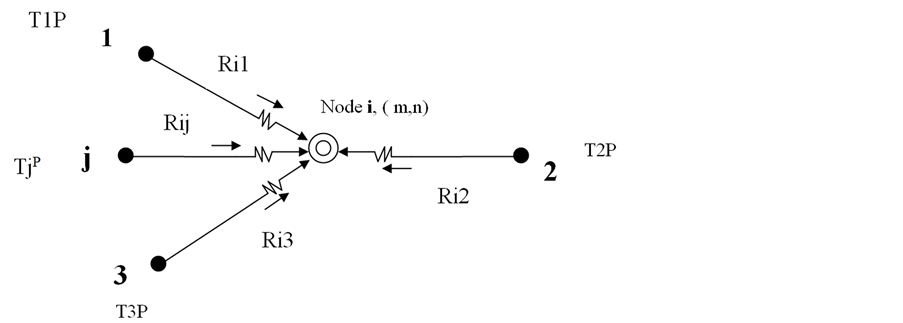
Figure 1. Inflow of heat to a node point.
DVi is the elemental volume. Ci is the heat capacity where Ci = ρi ci DVi; Dt is the time interval.
DE is the increase in the internal energy of the element; qi is the generated heat, if any, at point i.
Setting the sum of the energy (conducted, convected or radiated) into the node equal to the increase in the internal energy of the node, this energy-intake by the point is indicated by the temperature rise within the short interval of time.
In a steady-state, the net sum is zero, i.e. the net energy transfer is zero, while for the unsteady-state problems of our interest, here, the net energy-transfer into the node must be evidenced as an increase in internal energy of the element.
Thus: (2)
(2)
So that the general resistance-capacity formulation [8] , on the node, is expressed as:
 (3)
(3)
Under steady state condition Equation (3) becomes:
 (4)
(4)
3. Modeling the Temperature Generation at a Node Point
In a particular combustor model (Figure 2), of the following dimensions: External diameter = 72 cm, Wall
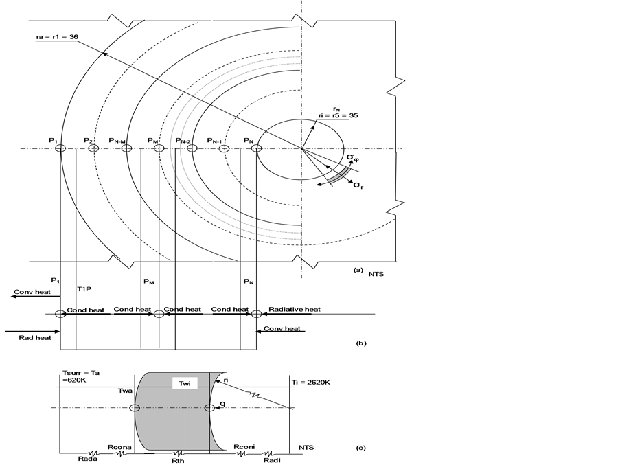
Figure 2. The cross-section of combustor. ri = inside radius of cylinder. ra = center of cylinder to outside surface.
thickness = 1 cm, and total length of 100 cm, this work is concerned with node point 1, P1, how its temperature is changing during the period of the transient thermal loading of the model combustor.
The compressor discharges directly to the combustor, where initially the bulk discharge volume is designed to divide into two streams: the greater stream goes into the annular space between the liner walls and the casing. This annular space can be equally designed as to determine the flow velocity, and thereby the convective heat transfer. With reference to Figure 2(c) the bulk stream temperature enveloping the liner, say temperature surrounding, Tsurr = 620 K.
The radiative heat resistances for inside and outside bulk streams are noted as Radi and Rada respectively. The heat capacity, C1:
 (5)
(5)
rm = radial position to center of nodal element; rm = conductive thermal resistance in material.
Δφ = polar angular measurement: Δφ = 2π, by full circular measurement.
Δz = incremental axial distance: Δz = 1 m, by full axial measurement.
ΔV = elemental volume, expressed in [μm3]. ;
; 
3.1. Parameter Information for a Nodal Equation
We assume on the outer surface a variable heat convection coefficient, ha.
 (6)
(6)
where h = a chosen constant coefficient: .
.
We also assume in the model material,

ha is chosen to vary as the temperature difference across the node at the transient time interval.
 , the conduction heat coefficient.
So that the conductive resistance, Rmi:
At boundary points,
 And,
And, (7)
(7)
 is the conductive thermal resistance for the external nodal point.
3.2. Temperature Equation on Outside Wall-Node Point 1
Temperature equation for Boundary point, Node 1:
Generally, the change in internal energy of a nodal element is given by
![]()
And the rate of change of internal energy , Where
  = the transient time interval in seconds. The instantaneous inflow of heat energy to a nodal element equals to the rate of change of internal energy.
For boundary point, Node 1: Analyzing the thermal resistances and balancing the transient energies:
Resulting
 (8)
(8)
where Tsurr = the bulk temperature of the surrounding, i.e. the peripheral Air stream temperature.
T1P = the nodal temperature before inflow of energies, T1(P+1) = the instantaneous new arrived temperature of the node, after receiving the inflow of energies.
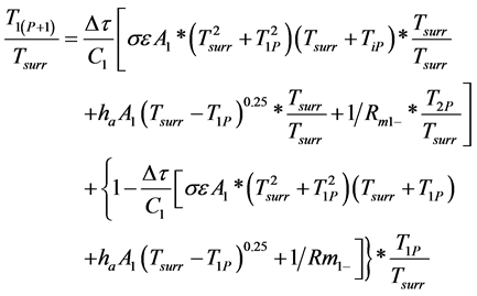
Expanding Equation (8),
 (9)
(9)
Equation (9) is the surface temperature equation.
3.3. Parametric Temperature Curves-Buckingham ( Theorem
Equation (9), the surface temperature equation can be further expressed in a non-dimensional form by dividing the whole function by the surrounding temperature, Tsurr:
That is,
 (10)
(10)
Expressing all Independent Parameters in Equation (10), the Buckingham π Theorem can be applied to give result in a non-dimensional function, as:
 (11)
(11)
Where  (12)
(12)
And  (13)
(13)
With  (14)
(14)
 (15)
(15)
And  (16)
(16)
Calculating the average heat transfer parameters.
 (17)
(17)
Numerically and typically, for Var 1.1, i.e. model combustor wall thickness of 2.5 mm Bcond = 0.8714 = constant, Bconv = 0.0001 = constant, Brad = 0.0037 = constant,
 (18)
(18)
Graphical presentation:
Temperature values (non-dimensional) T1(P+1)/Tsurr can be seen in the results of Program EU405TIPI for all Variants.
4. Results and Discussions
Non-Dimensional Outer Wall Surface Temperatures
The external node point temperature equation (wall surface) was expressed in a non-dimensional parametric form (by dividing through by the surrounding temperature, Tsurr, and applying Buckingham p theorem). Listing out the independent parameters involved, a temperature functional relation was expressed as:
 (19)
(19)
using Equation (10). This is the required surface temperature equation (non-dimensional).
In Figure 3, the results for computing non-dimensional outer wall surface temperatures for Var 4.1 (2.5 mm wall thickness) are shown. This non-dimensional expression involved the different modes of heat transfer, affecting the outer nodal point. Since it is an intrinsic line, Figure 4 shows the outer wall temperature at any particular time of C-variation.
Figure 5 shows the non-dimensional outer wall surface temperatures as plotted against the non-dimensional temperature parameter, Ca (Var 4.1). A determining line was found in order to make use of the graphical presentation of outer wall surface temperatures. This line was determined and worked out in a computer program, (EU405T1P1). Other results are given in Appendix. As an intrinsic line, this line turns out to be very important as it fixes the temperature at the instance of Ca variation. In Table 1, equation of change of outer wall surface temperatures was shown against the individual wall thickness.
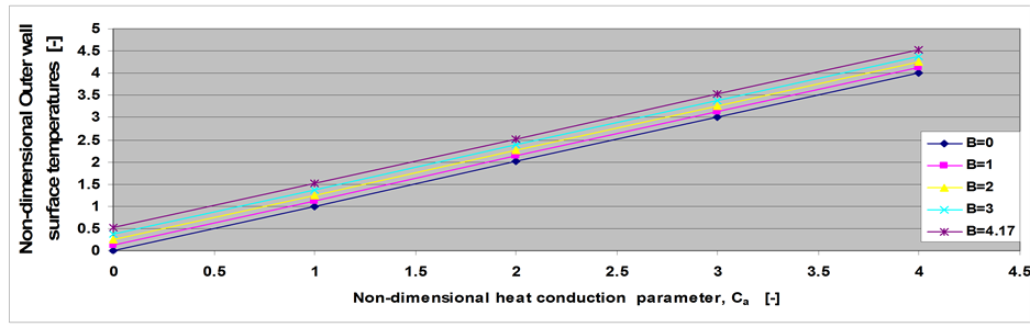
Figure 3. Outer wall surface temperatures (non-dimensional) versus non-dimensional heat conduction parameter Ca (Var 4.1), B = temperature ratio parameter: T1P/Tsurr.
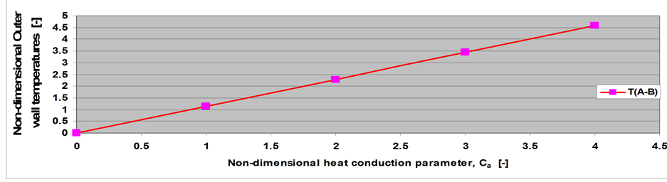
Figure 4. Variation of non-dimensional outer wall temperatures with heat conduction parameter, Ca, for wall thickness of 2.5 mm (Var 4.1).
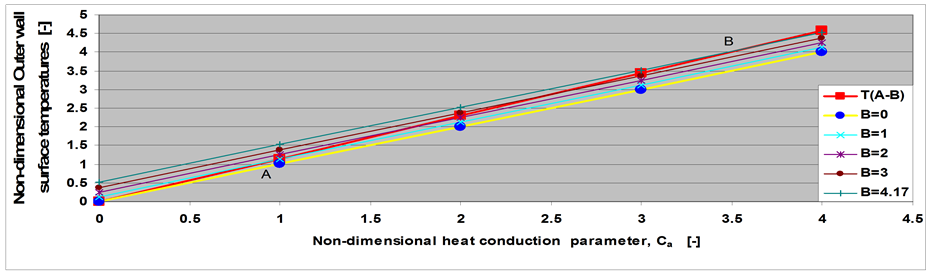
Figure 5. Outer wall surface temperatures (non-dimensional) versus non-dimensional temperature parameter Ca (Var 4.1)- showing lines of B = constant as straight lines. The intrinsic determinant line, AB is shown cutting across the parallel line graphs.

Table 1. Variation of equations of the change-rate of outer wall surface temperatures with non-dimensional temperature parameter, Ca (by Wall thickness).
5. Conclusion
The work has shown the method of generating wall-surface temperatures. Equation (10) generates in ordinary values, while Equation (18) generates non-dimensional values. In achieving this development, it has involved all the infuencing thermal conditions of the conductive, convective and the radiative heat transfers. The work has further shown that temperature generation follows an intrinsic trend line that is distinct to the wall-thickness concerned. Knowing the range of temperatures in application, this method can be recommended for use in confirming the suitability of a material when it will be put in application.
References
- Gilbert Gedeon, P.E. (2013) Nuclear Plant Material Selection and Application. Course No: T05-001 Credit: 5 PDH Continuing Education and Development, Inc. 9 Greyridge Farm Court Stony Point, New York.
- Yun, N., Jeon, Y.H., Kim, K.M., Lee, D.H. and Cho, H.H. (2009) Thermal and Creep Analysis in a Gas Turbine Combustion Liner. Proceedings of the 4th IASME/WSEAS International Conference on Energy & Environment, Cambridge, November 2009, 315-320.
- Jayakody, S. (2009) Why Is Selection of Engineering Materials Important? http://www.brighthubengineering.com
- Ufot, E. (2013) Modeling Thermal Stresses in Combustor of Gas Turbines. Ph.D. Thesis, Rivers State University of Science and Technology, Port Harcourt.
- Tinga, T., van Kampen, J.F., de Jager, B. and Kok, J.B.W. (2007) Gas Turbine Combustio Liner Life Assessment Using a Combined Fluid/Structural Approach. Thermal Engineering, Twente University, Enschede.
- Elsner, N. (1975) Grundlagen der Technischen Thermodynamik. 3rd Edition, Akademie-Verlag, Berlin.
- Hart, H.I. (2005) Engineering Thermodynamics, a First Course. King Jovic Int’l, Port Harcourt.
- Holman, J.P. (1997) Heat Transfer. 8th Edition, McGraw-Hill, Inc., New York.
Nomenclature
A1: convective and radiative heat transfer external surface area [m2]
AN: convective and radiative heat transfer internal surface area [m2]
ha: convective heat transfer coefficient for external wall surface [W/m2×K]
hi: convective heat transfer coefficient for internal wall surface [W/m2×K]
k: conductive heat transfer coefficient in the material [W/m×K]
q: Transferred heat from the inner bulk fluid stream through the [kJ]
material wall to annular space ri: radius to inner wall surface from center of cylinder [m]
ra: radius to outer wall surface [m]
Rac: sum of outer radiative and convective resistances [K/W]
Ric: sum of insde radiative and convective resistances [K/W]
Rada: radiative heat resistances for outside wall [K/W]
Radi: radiative heat resistances for inner wall [K/W]
Rcona: convective thermal resistances for outer wall [K/W]
Rconi: convective thermal resistances for inside wall [K/W]
Rth: conductive thermal resistances in material [K/W]
Rtotal: total thermal resistance of the system: [K/W]
Ta: constant outer surrounding temperature, Ta = Tsurr [K]
Ti: internal bulk stream temperature [K]
Twa: outer wall surface temperature [K]
Twi: internal wall surface temperature [K]
Tsurr: the surrounding temperature, main annular temperature [K]
Greek letters:
ε emissivity
σ Stefan-Boltzmann constant [W/m2∙K4]
Suffixes
th thermal z distance in axial direction
Appendix. Computer Program for the Computation of the Surface Temperatures
Code(using Visual Basic language): EU405 “T1P1/Tsurr-FUNCTION RESULTS-EU405 T1P1/Tsurr EU405-T1P1/Tsurr Function PROGRAM RESULTS
DT = 0.014 ra = 35.25 cm Thickness = 2.5 mm Brad = 0.0037 Bcond = 0.8714 = const Values of T1P1/Tsurr Bconv = 0.0001 B C0 C1 C2 C3 C4
1.0 0.13 1.13 2.13 3.13 4.13
2.0 0.25 1.25 2.25 3.25 4.25
3.0 0.38 1.38 2.38 3.38 4.38
4.2 0.52 1.52 2.52 3.52 4.52 Slope Calculation Results Twa, F, Bmax, X, Y, Cend, x1, y_c1, mx, m 2583.1 4.17 4.17 0.00381 0.12482 3.6424 2.6 1.007 0.057 1.1426 y = mC + yo; yo = 0.0044
NOTES

*Corresponding author.