Engineering
Vol.4 No.12A(2012), Article ID:26080,6 pages DOI:10.4236/eng.2012.412A122
Influence of the Chemical Composition of Completion Fluids on the Propagation of Electromagnetic Waves within Oil Wells
Departamento de Engenharia Elétrica, Pontifícia Universidade Católica do Rio de Janeiro, Rio de Janeiro, Brazil
Email: ashade@ele.puc-rio.br
Received August 15, 2012; revised September 22, 2012; accepted October 4, 2012
Keywords: Electromagnetism; Oil Well; Wireless Telemetry; Monte-Carlo; Uncertainties; Heterogeneous Media
ABSTRACT
The propagation of electromagnetic waves in the annular region of oil wells was studied. The present study aims to analyse the propagation attenuation along the well, as well as the input impedance determined by a source placed near the wellhead. A coaxial waveguide model was adopted with heterogeneous dielectrics and losses. First, a wave equation solution for the waveguide is presented, assuming a homogeneous medium with losses, by solving the equation in cylindrical coordinates using the vector potential technique. An uncertainty analysis model is then developed to model the heterogeneous characteristics of the medium. Monte Carlo simulations were performed with the created model using data gathered from the literature. The results of the simulations indicate that propagation in the transverse electromagnetic mode has the smallest attenuation and that for depths of up to 4000 m, there is an attenuation of less than 52 dB. Furthermore, the input impedance ranges from 10 Ω to 10 kΩ because of the uncertainties involved in the problem in question.
1. Introduction
Oil wells today are extremely complex and demand very expensive maintenance [1]. Modern drilling techniques can reach a few kilometres in depth, and the costs of a floating platform at open sea can cost billions of Brazilian Reais. Thus, it is critical to determine the internal conditions of the well, and indicators such as temperature, pressure and salinity must be constantly monitored [2].
Reliable telemetry by cables is very difficult to obtain due to the extreme conditions of the internal environment of an oil extraction well. As an example, there is continuous abrasion by sand and dirt that are carried by fluid flow. For this reason, the cables are periodically damaged and require replacements. Such replacements hinder the oil extraction process and, moreover, increase the costs due to the large amount of cables needed over the life of a single well.
The most obvious alternative to cabling is the adoption of wireless telemetry. However, the amount of electricity required to power wireless communication is not practical: power cables are needed because the use of batteries would lead to frequent maintenance, as they need to be recharged [1]. It is obvious, therefore, that the objective (and greater challenge) is to build a system without wires or batteries; that is, the downhole sensors must be powered and communicate with the base without the use of cables.
Several approaches are possible for wireless telemetry. One possibility would be the use of signal transmission techniques using a magnetic field [3]. In this method, a coil that is capable of inducing alternating current through the production pipe is used. This coil has sufficient intensity to transmit both power and the signal itself between the sensor and the base [4]. Through a second coil positioned at the sensor location, it is possible to recover the signal and power needed to feed and produce bilateral communication. However, the technique has a weakness: the production tube is not a transformer core, i.e., it is not designed to minimise the magnetic flux losses. Its hollow characteristic confers much loss by parasitic Foucault currents concomitantly with hysteresis losses, the cause of which is due to the inadequacy of the production tube material for magnetic purposes [5]. Therefore, for long distances, on the order of 3000 m or more, the method is unfeasible.
Another possible approach would be to analyse the oil well from the perspective of a coaxial propagation structure, which is formed by a conductor tube with a perfect centre (production tube) and a cylindrical shell that is coaxial with the tube and is also a perfect conductor. This approach makes it possible to conduct the analysis as it would be performed on a coaxial cable, and therefore, propagation occurs in the transverse electromagnetic mode [6]. This approach, however, has been studied without considering fluids of significant conductivity or possible uncertainties caused by temperature and electrical parameter variations of the fluid that fills the well.
The modelling difficulty concerns the fluid that fills the well. This fluid is heterogeneous because it exhibits significant variation in electric permittivity along the well depth. Furthermore, the actual fluid concentration varies from well to well, and at times within the well itself, which is another source of heterogeneity.
In this context, the present article proposes to study the electromagnetic propagation inside the annular area of oil wells. The goal is to develop a model that permits an approximation of the behaviour of the TEM propagation mode in the coaxial structure with losses and the previously cited heterogeneous characteristics. The first step is the deduction of the electric and magnetic field equations within the well, assuming a typical well structure. Thereafter, statistical models of the parameters that compose the medium are developed, considering their temperature variations and propagation frequency. Finally, the study uses Monte Carlo analysis to illustrate how the propagation attenuation behaves and to analyse the input impedance of the coaxial waveguide as a function of position.
2. Modelling
2.1. Well Definition
The well will be modelled according to Figure 1. This
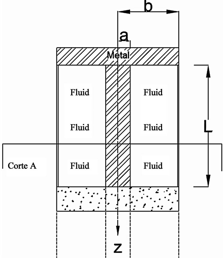
Figure 1. Adopted well structure. A semi-infinite well is assumed and is formed by two concentric cylinders and a metal block covering the top of the waveguide.
figure depicts a coaxial guide bounded by perfect conductor metals with a homogeneous dielectric and losses. The upper extremity is completely closed by a perfect conductor metal to model the valve and metal duct assembly present in a wellhead. The bottom of the well is composed of concrete; however, this fact is neglected, and the well is assumed to behave as a semi-infinite waveguide.
2.2. Deduction of the Propagation Equations
Modelling is performed using Maxwell’s equations and the concept of vector potentials. The Maxwell’s equations used are Equations (1) and (2):
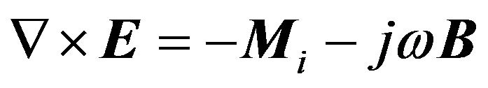 (1)
(1)
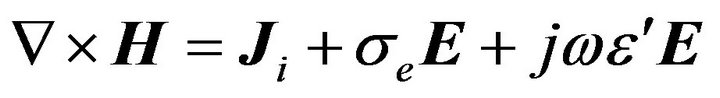 (2)
(2)
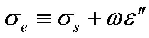
The real number constant  is the real part of the complex electrical permittivity of the medium. Furthermore, the complex constant σe is called effective conductivity and it represents the linear relation of conduction current and electric field on the medium.
Consider a medium with no source of magnetic charge  . Because
 , the curl of A can be defined as
 (3)
(3)
Substituting 3 in 1 and considering Mi = 0 (Induced magnetic flux equal to zero), we obtain:
 (4)
(4)
Or:
 (5)
(5)
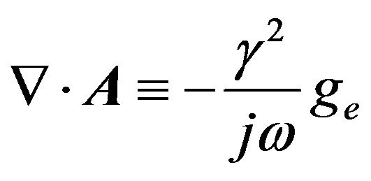
Since  , an electric scalar potential ge can be defined such that:
 (6)
(6)
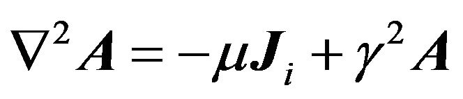
Applying the identity  in Equation (3) and using Equation (2), we obtain:
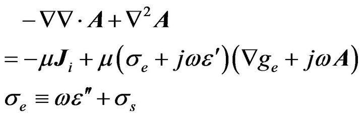 (7)
(7)
In Equation (7), the parameter σe is the effective conductivity of the medium, while σs represents the static conductivity, that is, the conductivity when frequency is zero. At this moment, we are in a position to define  . To simplify Equation (7), we use the gauge:
 (8)
(8)
where  is the complex constant of propagation of the medium. This step simplifies the equation for the electrical potential, resulting in:
 (9)
(9)
For homogeneous media, Equation (9), when solved, determines the electric vector potential in the medium, which can be used to obtain the equation for the electric field as a function of the electric vector potential:
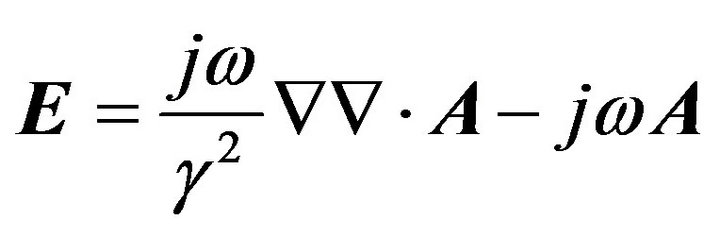 (10)
(10)
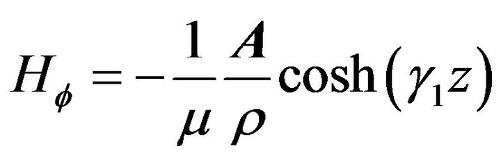
We seek the solution in transverse electromagnetic mode (TEM), which is generated using with the restriction Ez = 0, which leads to the following fields in cylindrical coordinates:
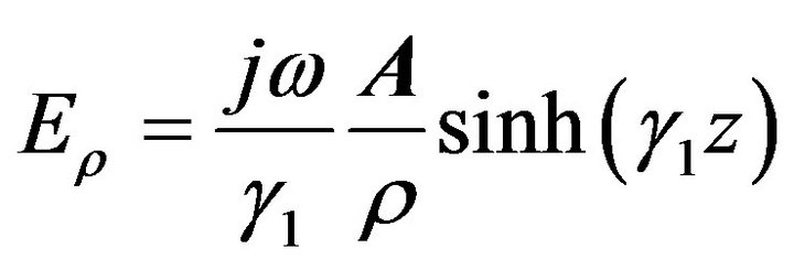 (11)
(11)
 (12)
(12)
 (13)
(13)
Note that because EΦ = Ez = 0, the boundary conditions that require a null tangential component in the metal extremities are already met. As the well has a metal structure at one of the extremities, one must also ensure that Eρ (z = 0) = 0. Note, however, that this condition is also already guaranteed.
The above solution represents a propagation model in TEM mode in a coaxial medium with losses inherent to the medium inside. However, it is important to remember that the solution was obtained by assuming a homogeneous propagation medium.
2.3. Statistical Modelling of the Medium Constituent Parameters
The propagation medium in the well consists of an oilbased dielectric fluid composed of water, oil and salts (typically CaCl2) [7]. This fluid is the centre of all electromagnetic propagation, and therefore, its electrical characteristics must be examined in detail. A study over the range of 1 MHz to 100 MHz was previously conducted [7], revealing significantly variable behaviour based on the chemical composition of the fluid.
To model the variation of conductivity with frequency, the effective conductivity concept is applied [8] using the following formula:
 (14)
(14)
From the experimental curves obtained in [8], the parameters  and
and  can be calculated using a least squares method.
An analogous model can be created to model the variation in frequency of the real relative permittivity with the frequency. With
 (15)
(15)
and using the experimental curves in [8], it is possible to estimate the parameters and ![]() using a least squares approach.
using a least squares approach.
In addition to the variation in frequency, variation in the medium  constituent parameter can also be observed in temperature. Such variation cannot be neglected because inside a 5000 m deep well, it is impossible to ensure that the temperature is uniform along its entire length. This fact, therefore, characterises non-homogeneity along the z direction.
To circumvent the situation, a model that assumes an average temperature in the medium is adopted. This temperature, in turn, is considered constant throughout the well, which implies a homogeneous medium. Thus, the influence of the variation of this average temperature on signal propagation in the well can be analysed, assuming a valid range of average temperatures.
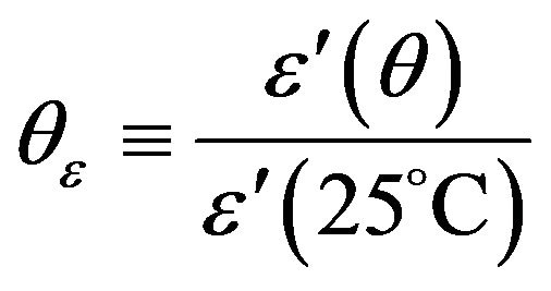
Mathematically, a coefficient of correction in temperature is defined as the ratio between the temperature value in question and the value of the reference temperature, here defined as 25˚C. Thus,
 (16)
(16)
 (17)
(17)
 (18)
(18)
The quadratic form was selected to present the best interpolating results using the experimental data from [8].
Similarly, there is increasing variation in the relative permittivity according to the temperature, as demonstrated by [7]. Again, it is used a quadratic model similar to the effective conductivity variation in temperature:
 (19)
(19)
 (20)
(20)
 (21)
(21)
3. Experiments and Results
In all the experiments, a well with a length of 5000 m, an inner radius of 0.05 m and an outer radius of 0.1 m is assumed. All the Monte Carlo analyses were conducted with at least 1 million samples. The objective of the experiments was to obtain graphs and numerical values for the input impedance of the “oil well” waveguide and to analyse the propagation loss in the medium for 5000 m of depth.
All analyses were conducted over the range of 1 MHz to 100 MHz. For the other free parameters, the modelling used random variables whose distribution was selected to reflect their most common values. Table 1 summarises the values selected for each free parameter of the previously described model and their respective distributions. For simplicity, when the random variable has simple and obvious domain restrictions, a uniform distribution was selected; otherwise, a normal distribution was used. Furthermore, statistical independence was assumed between the variables.
First, an experiment was conducted to calculate the attenuation in the well. The attenuation is directly dependent on the real part of the constant of propagation, whose square is defined as 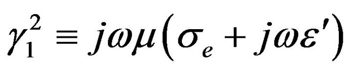 .
.
The models proposed in Section 2.3 were used for the conductivity and electric permittivity, and the relative magnetic permeability was assumed to be equal to 1.
The Figure 2 presents a boxplot of the constant of attenuation for the various frequencies between 1 and 100 MHz. Values that appear in the graph as outliers are from highly unlikely combinations of the random variables of the problem and are most likely not physically feasible and, therefore, must be disregarded. The height of the boxes represents the range of values most likely to be observed, and its average point is a good approximation of the average. The boxplot of Figure 3 demonstrates that the attenuation constant increases with an increase in frequency, as expected. Furthermore, note that the deviation of the coefficient increases with the elevation of the propagation frequency, which makes the system design even more difficult. Thus, it is clear that lower frequentcies are desirable from the point of view of signal attenuation.
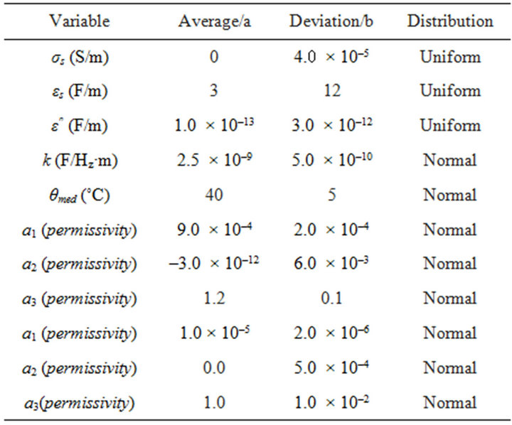
Table 1. Random variables used for modelling uncertainties. For simplicity, when the random variable has simple and obvious domain restrictions, a uniform distribution was selected; otherwise, a normal distribution was used.
Using the TEM mode equations presented in Equation (2), it is clear that the wave propagating in the direction of the bottom of the well has power attenuation given by 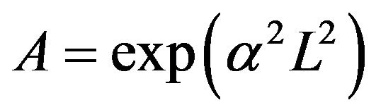 . Using the statistical analysis of the coefficient of attenuation, Table 2 was generated.
The values from the table represent the upper limit of attenuation for 95% of the cases. Thus, for example, for a depth of 1000 m, P (A ≤ 13 dB) = 0.95. The results presented in Table 2 do not agree with the propagation for L = 5000 m of depth because of the high-energy attenuation (130.3 dB). However, it is essential to note that the table represents an upper limit of attenuation, taking 95% of the possible combinations of propagation medium and an average temperature. Moreover, as the table demonstrates, propagations up to 2000 m depth are highly acceptable, as an attenuation of up to 52.1 dB is observed in current communication technology. Even at greater depths, the possibility of communication cannot be excluded.
The second experiment was performed to analyse the input impedance of the coaxial waveguide as a function of the excitation source position. The experiment was conducted at 1 MHz.
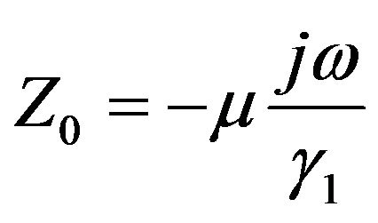
Setting the impedance at any point as the ratio , we obtain
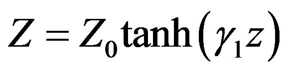 (22)
(22)
 (23)
(23)
 (24)
(24)
The position selected for analysis was at  wavelength from the wellhead, that is,
  . However, the wavelength itself is a random variable because
  and
and  is a random variable. Monte Carlo analysis revealed that
 ![]() varies between 90 m and 170 m for 90% of the cases, leading to the selection of position
varies between 90 m and 170 m for 90% of the cases, leading to the selection of position 
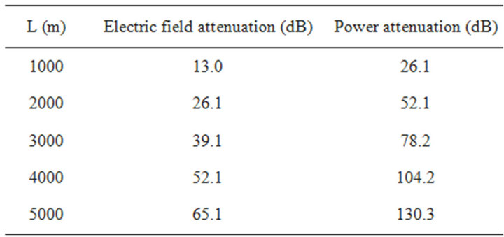
Table 2. Estimated attenuation of electromagnectic waves propagating in the annular region of the well.
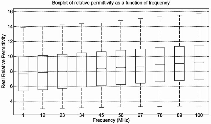
Figure 2. Boxplot of relative permittivity as a function of frequency. The horizontal axis represent the frequency of propagation in MHz, while the vertical axis represent the actual value of the electrical permittivity.
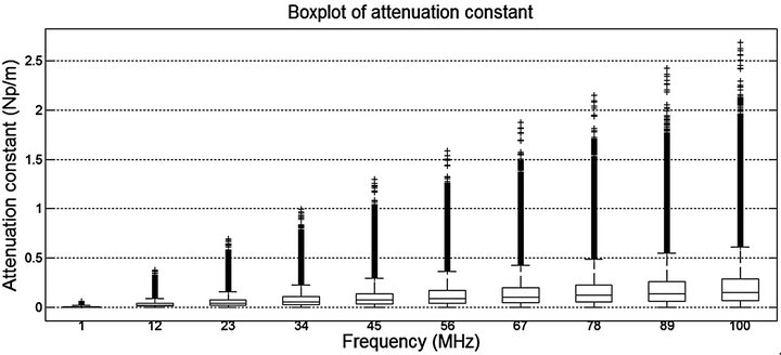
Figure 3. Boxplot of attenuation constant as a function of frequency.
Using Monte Carlo analysis again, it can be observed in Figure 4 that the input resistance (real part of the impedance) of the system exhibits great variation, ranging from 10 Ω to 1.0 kΩ for 90% of the cases. This variation is due to the variation of the relative permittivity in the medium. Therefore, it is necessary to design a generator circuit that provides a good match for a wide range of input impedances, i.e., the generator/receiver circuit must lose as little power as possible by reflection.
4. Conclusions
The present study focused on analysis of the electromagnetic propagation inside the annular area of oil wells, assuming the interior medium is composed of dielectrics with significant conductivity. The well behaviour was evaluated with respect to the input impedance and propagation attenuation.
To quantify the well behaviour with respect to electromagnetic propagation, a coaxial waveguide model was developed, modelling the wellhead as a metal cap that completely closes one extremity of the waveguide. First, we solved the wave equation for a homogeneous cylindrical coaxial waveguide, resulting in an analytical model. Then, an uncertainty model was adopted to approximate the heterogeneous and imprecise characteristics of the fluid that functions as a dielectric inside the well.
Using this model, two experiments were developed, both by simulation. The first aimed at analysing the input impedance observed by a source positioned at 1/4 of the wavelength from the wellhead, while the other aimed at analysing the attenuation as a function of length or well depth.
Due to the uncertainties present, the input impedance
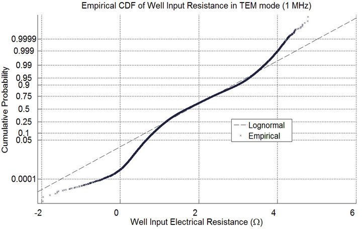
Figure 4. Empirical cumulative distribution function of the well input resistance in TEM mode at 1/4 wavelength from well head. The horizontal axis show the log on base 10 of the value of input resistance in Ohms, while the vertical axis show the cumulative distribution function value.
was observed to vary from 10 Ω to 1 kΩ for the frequency of 1 MHz. The conclusion was obtained by Monte Carlo simulation and was applied to the expression derived for the waveguide input impedance.
By performing the attenuation analysis, it was concluded that for 95% of the cases, the constant of attenuation in TEM mode is less than  Np/m for a frequency of 1 MHz. The power attenuation at 4000 m depth was also observed to be approximately 100 dB for the same frequency of 1 MHz, with 95% probability. Although 100 dB appears to be a large attenuation, most wells in operation are between 1000 m and 2000 m in length, and the attenuation is much lower at these depths.
REFERENCES
- S. Brilles, “Remote Downhole Well Telemetry,” US Patent US6766141, 2004.
- J. A. D. Rosa, A. J. Carvalho and R. D. S. Xavier, “Petroleum Reservoir Engineering,” Rio de Janeiro, 2006.
- F. Sakata, H. Wakiwaka, M. Hanabusa, N. Yamazaki and H. Yamada, “Performance Analysis of Long Distance Transmitting of a Magnetic Signal in a Cylindrical Steel Rod,” IEEE Translation Journal on Magnectics in Japan, Vol. 8, No. 2, 1993, pp. 102-106.
- F. Harold J. Vinegar, R. R. Burnett, G. C. W. M. Savage and J. W. Hall, “Permanent Downhole, Wireless, TwoWay Telemetry Backbone Using Redundant Repeaters,” US Patent US6633236B2, 2003.
- B. W. Kennedy, “Energy Efficient Transformers,” New York, 1998.
- K. A. Safynia and R. W. McBride, “System and Method for Communicating Signals in a Cased Borehole with Tubing,” US Patent US4839644, 1989.
- P. A. Patil, et al., “Experimental Study of Electrical Properties of Oil-Based Mud in the Frequency Range from 1 to 100 MHz,” SPE Drilling and Completion, Vol. 25, No. 3, 2010, pp. 380-390. doi:10.2118/118802-PA
- C. A. Balanis, “Advanced Engineering Electromagnetics, Vol. 52, No. 1,” Wiley, Hoboken, 1989, p. 1008.