Engineering
Vol. 4 No. 10 (2012) , Article ID: 23361 , 4 pages DOI:10.4236/eng.2012.410081
An Experimental Study on a Characteristics of Flow around Groyne Area by Install Conditions
Department of Water Resource Research, Korea Institute of Construction Technology, Goyang, South Korea
Email: jgkang02@kict.re.kr, yeo917@kict.re.kr,csckim@kict.re.kr
Received July 25, 2012; revised August 27, 2012; accepted September 8, 2012
Keywords: Low Drop Structure; Local Scour; Physical Habitat; Scour Size
ABSTRACT
In designing group groynes, the space of the groynes is an important factor, and the flow between the groyne areas will vary along the space. Since the flow in the groyne field significantly affects the flow change, the bed change, the bank erosion and the condition of the habitat, an assessment of the flow along the space of the groynes will yield important data needed to diversify the object of the groyne installation. To provide basic data for the determination of the proper space of groynes in a groyne group, the flow in the channel and groyne field, which varies with the installation of the groyne, is herein analyzed. The space of the groynes was set from the same length to 12 times the length of the groyne, and the flow range was measured using the LSPIV method and ADV. The influence of the angle of the installation was also analyzed. As a result, through the flow configuration in the groyne field and the flow range at the center of the groyne field against the space of the groyne, the decreasing influence of groyne erosion was suggested by the analysis of the shelter effect of aquatics and the countercurrent in the bank line.
1. Introduction
A groyne is a structure installed in the front part of a bank or a bank line for protection, flow control, ensuring of the depth of the main channel, etc. Recently, the purpose of groyne installation has varied due to the issue of environmental functions in which the countercurrent in the groyne field and the recirculation zone provide various habitats to aquatics and shelters during floods, etc. There are various main design factors such as the space of the groynes, the direction (angle), the height, the length, the bad condition, the flow characteristics, etc. Especially, in the case of group groynes as shown in Figure 1, the assessment of the flow along the space of the groynes is the key factor in the design of groynes because the flow in the groyne field significantly affects the flow change in the groyne field, the bank line erosion, and the habitat condition.
A previous study on the space of groynes suggests that “the space of groynes may have to be maximized to properly protect the bank line” and its space (L), the length of the groyne (l) and its non-dimensional value (L/l). Acheson [1] suggested the space L/l = 2 - 4 for the angle of curvature, but failed to support a precise standard for the relationship between the space of the groynes and the groyne transmissivity and curvature. Fenwick [2] classified the space of the groynes according to the purpose of their installation (for example, L/l = 2 - 2.5 for flow control and L/l = 3 for bank protection). Richardson and Simons [3] suggested L/l = 1.5 - 2.0 and L/l = 3 - 6 along the condition of installation (for instance, 4 - 6 for a straight line or a curved groyne with a large radius and 3 - 4 for a curved groyne with a small radius). Jansen et al. [4] suggested the inclusion of the space of the groyne in the energy Equation (1) based on the results of their irrigation experiment.
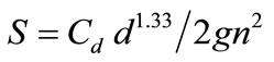 (1)
(1)
The energy loss coefficient Cd yielded by the experiment performed herein was 0.6. The above equation shows a big space, and Kinori and Mevorach [5] suggested that this value be applied as an upper limit.
Copeland [6] suggested no less than L/l = 3 using the length of the groyne erosion for bank line protection. FHWA [7] suggested considering the length, angle, transmissivity, and curvature of the curved channel of the groyne, the general range of which was L/l = 1 - 6, for the purpose of groyne installation and protection. The results of the research of FHWA expressed the length of the bank protected by each groyne into the flow extension angle, which indicates the angle from the vertical hem of the groyne to the line of the groyne that ends the recirculation zone. An extension angle of 17 degrees was suggested for non-transmissive groynes, and the exten-
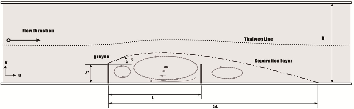
Figure 1. Sketch of flow area between two groynes.
sion angle increased with the transmissivity in the transmissivegroyne.
The previous researches show experimental results based on the installation purpose (groyne protection, flow control, etc.), but failed to suggest the data for the flow characteristics (the increasing flow velocity in the channel and the vortex phenomenon in the groynefield) at the channel and groyne fields along the space of the groynes. Thus, this study aims to analyze the influence of the flow along the space of the groynes and to derive data to suggest the space of the groynes through an irrigating model test.
2. Existing Studies
A flow profile measuring experiment along the groyne installation was directly performed in a 2.0 m (B) × 0.65 m (H) × 40 m (L) channel, as shown in Figure 2, and a 1.2 m-wide weir that supplied 0.012 - 0.4 m3/s was installed as the flux supplier. As shown in Figure 3, two identical groynes were installed at the center of the channel to determine the flow change around the groyne field along the space of the groynes. The length of the installed groynes was 0.3 m, the ratio to the channel width of which was 0.15, and the groynes were made of acrylic plastic. In a portion of the space of the groynes, the groyne length was set at 1 - 12. The flow conditions applied were 0.09 m3/s for the flux, 0.15 m for the depth, and 0.3 m/s for the approaching flow velocity. The LSPIV (Large-Scale Particle Image Velocimetry) and the ADV (Acoustic Doppler Velocimeter) methods were used to measure the flow velocity and the flow field in the groyne field, respectively. As shown in Figure 4, the mid-level flow velocity (60% of the water depth) was measured using the ADV method, and the result was averaged per minute.
In this study, the LSPIV method was applied to the measurement of the flow velocity field of the groyne field and the main flow of the channel, as shown in Figure 5. The LSPIV method is identical to the PIV method. Since it has the advantage of being able to overcome the
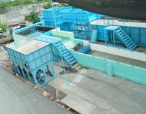
Figure 2. Experiment flume and water supply.
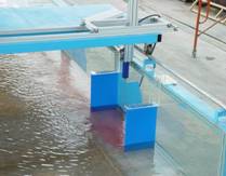
Figure 3. Experiment setup of groynes for L/l = 2.
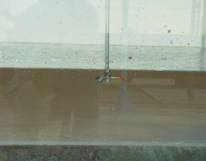
Figure 4. Measurement of velocity using ADV.
limit of LDV (Laser Doppler Velocimetry) and ADV and measure the instant flow velocity field at the overall target region, it is frequently used in local flow fields around
 (a)
(a) (b)
(b)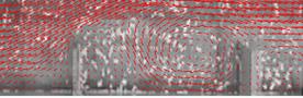 (c)
(c) (d)
(d)
 (e)
(e)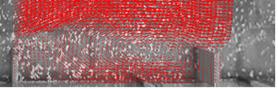 (f)
(f)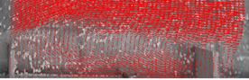 (g)
(g)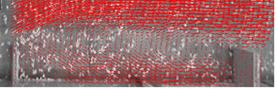 (h)
(h)
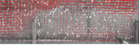
Figure 5. Velocity fields of groyne field measured by LSPIV. (a) L/l = 3; (b) L/l = 4; (c) L/l = 5; (d) L/l = 6; (e) L/l = 8; (f) L/l = 10; (g) L/l = 11; (h) L/l = 12.
groynes (Ettema and Muste [8] and Weitbrecht et al. [9]).
3. Channel with Groyne Installation and Flow Velocity Distribution of the Groyne Field
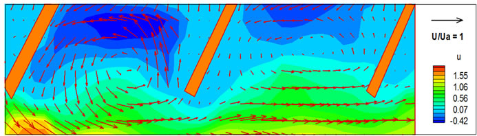
The flow in the groyne field for the space of the groynes was analyzed with respect to the flow shape of the groyne field along the space of the groynes and the backward flow, the vertical tip flow velocity of the downstream groyne, and the flow angle created along the bank line. The flow shape at the groyne field was assumed to have changed the shape of the vortex along the space, and was measured to determine various flow shapes caused by the installation of the groyne. The flow shape at the groyne field along the space showed a difference in the shape of the generated vortex. One vortex was generated at the ratio of the space of the groynes to the length of the groyne (L/l) of no more than 3, and two vortexes, at L/l = 3 - 7. The second vortex was deformed at L/l = 8 - 9, and three vortexes were generated at L/l = 10. It seems that the vortex generated at L/l = 3 was generated because the flow of the channel rotated the stagnant fluid at the back of the upstream groyne. However, when L/l was no less than 3, two vortexes seemed to have been generated because the fully developed clockwise backward flow that flowed along the downstream groyne created a boundary with the stagnant fluid at the back of the upstream groyne. The three vortexes generated were measured when L/l was no less than 10, and were determined to have been influenced by the recirculation zone and the downstream groyne. Figures 5 and 6 show the flow and the flow velocity field at the groyne field, measured with LSPIV.
The backward flow generated along the bank line was analyzed near the bank line (y = 0) and the sideline (y = 0.11), and the flow velocity rate non-dimensioned by the upstream approaching velocity was applied. The flow velocity of the bank line dramatically increased when L/l was more than 3, and the change in the flow velocity along the space of the groynes was measured. The flow velocity of the bank line at L/l = 1 and 2 was found to have been almost zero. The maximum flow velocity at the groyne field was found to have been around 0.5 when L/l = 4 - 12. When L/l = 4 - 7, the position of the maximum flow velocity was found to be at 0.8 of the space of the groynes; when L/l = 7 or more, it moved upwards; and when L/l = 12, the position of the maximum flow
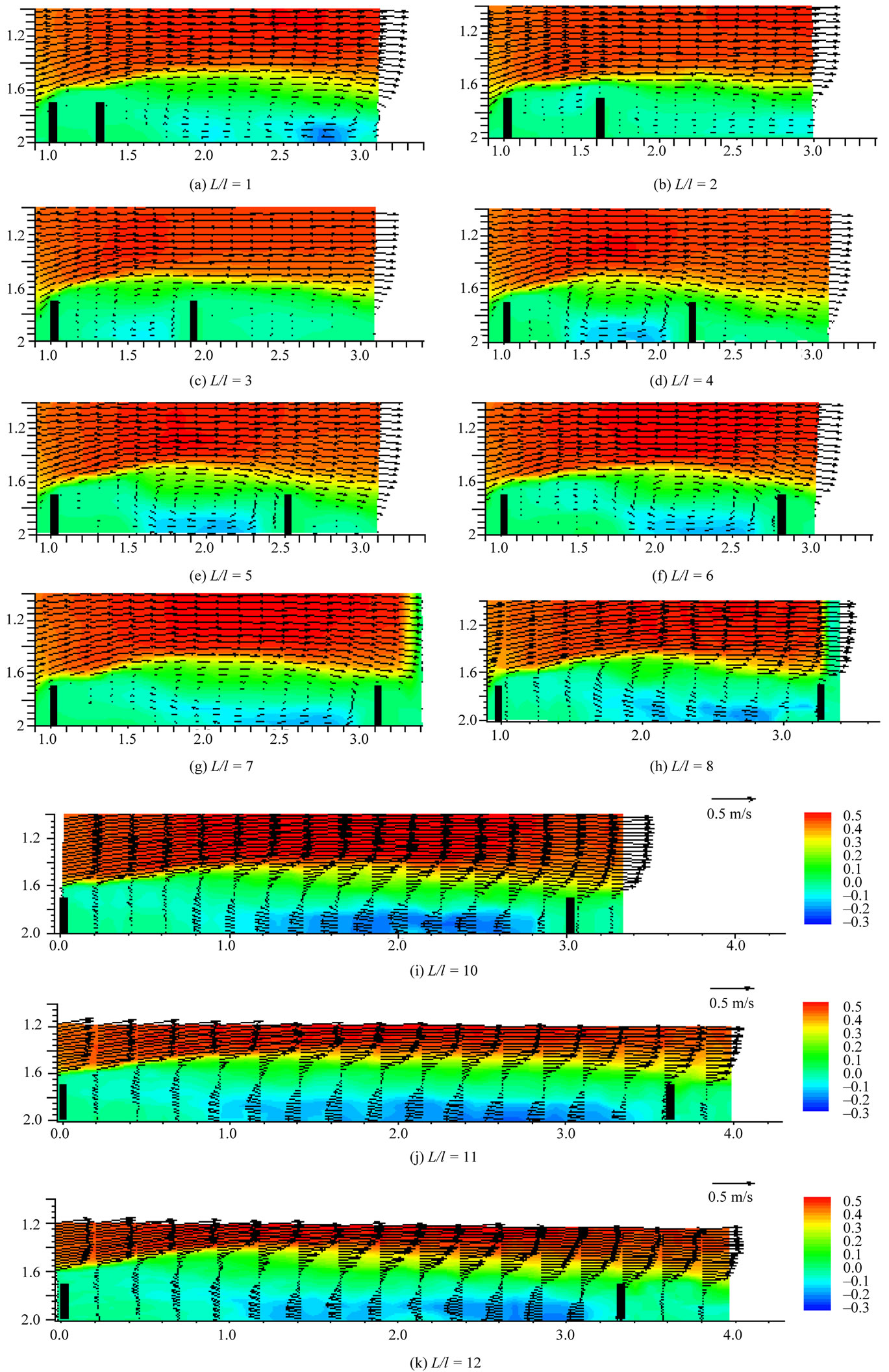
Figure 6. Velocity fields of groyne field measured by LSPIV.
velocity was measured at 0.4 - 5. For the flow velocity distribution (vertical direction), one variation point appeared at L/l = 3 - 7, but when L/l = 8, two variation points appeared. This phenomenon shows that from L/l = 8 or more, the flow changes because the vortex flow at the groyne field changes the flow pattern. The downstream vertical flow and its angle are shown in Figures 7 and 8. The downstream groyne vertical flow relatively increases along the space between the groynes and its angle also increases. The flow angle was measured to have moved counterclockwise. This phenomenon was found to have been caused by the influence of the backward flow generated at the recirculation zone in the upstream groyne field (Kang, Jungu et al. [10]).
4. Flow Analysis at the Groyne Field along the Groyne Installation Angle
Measurements of the vertical groynes (SF-90) at the cen-
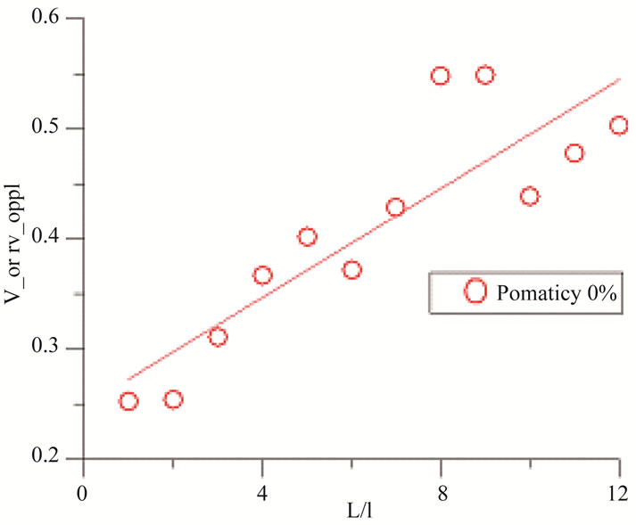
Figure 7. Relationship between groynes interval with tipvelocity of 2nd groyne.
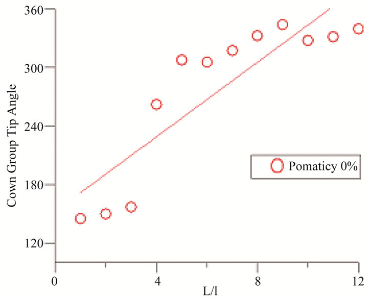
Figure 8. Relationship between groynes interval with tipflow angle of 2nd groyne.
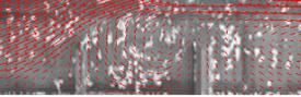
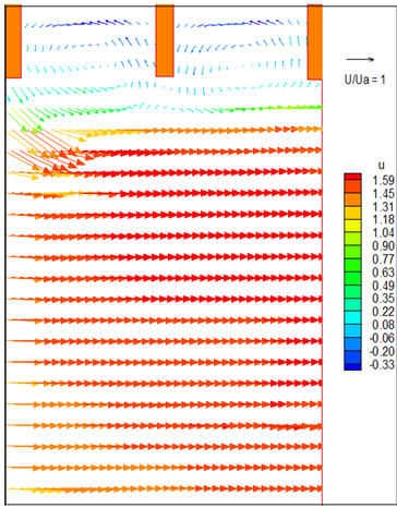
tral depth using ADV were simultaneously conducted to compare the LSPIV analysis data. Fried rice was used as the particle in the LSPIV method. The influence of the viscosity between the particles and the form rate was found to be negligible. In the case of the measurement using ADV, the grid point of 15 × 5 in the groyne installation area was measured and its averaged data for 60 seconds was used, and more resolution was added in the groyne field to compare the LSPIV analysis data. Figure 9 shows the surface flow pattern at the groyne installation area filmed with a video camera, as well as the flow vector, which was at the mid-level, using ADV. That is,
 (a)
(a)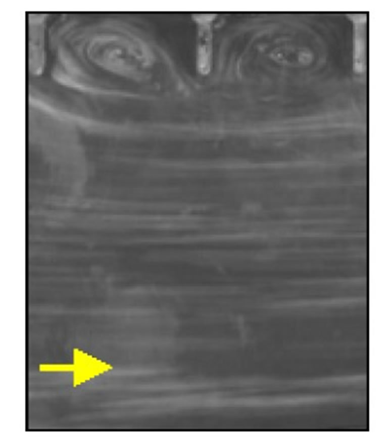 (b)
(b)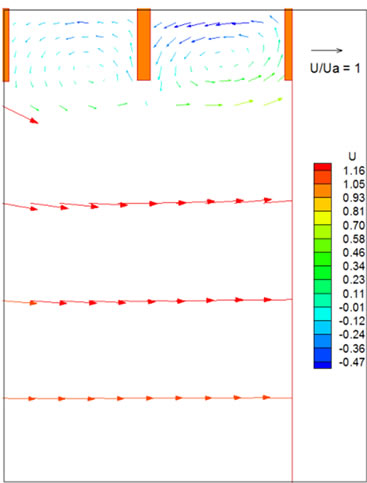 (c)
(c)
Figure 9. Flow pattern and velocity profile around install groyne area (SF152-90). (a) LSPIV data; (b) Video image; (c) ADV data.
in the experiment on SF152-90, the vertical groyne was = 0.15 and = 2. As shown in the video, a counterclockwise vortex flow existed at the upstream and downstream groynes, and flow separation generated at the upstream groyne influenced the flow pattern at the downstream groyne. The core of the vortex was located at the center of the groyne field, and the size of the vortex was bigger at the upstream groyne. The main stream beside the groyne field was mostly parallel to the channel, and the influence of the upstream groyne reached the length of the groyne in the horizontal direction.
From the result of LSPIV and ADV application, the velocity of LSPIV analysis is relatively smaller because of the difference of measuring point (surface and midlevel) but its trend of velocity distribution is determined to be well coincident at groyne and main channel. For upstream and downstream groyne, surface flow velocity was achieved with application of LSPIV and its part of result is shown in Figures 10 and 11, the space of groynes is 4 times bigger than the length, 2 vortex are shown
 (a)
(a)  (b)
(b) (c)
(c)
Figure 10. Flow pattern around install groyne area (SF252- 60/120). (a) SF252-60; (b) SF252-120; (c) SF252-90.
 (a)
(a)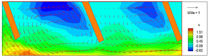 (b)
(b)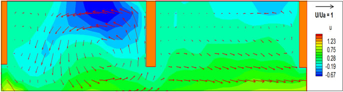 (c)
(c)
Figure 11. Velocity vector around install groyne area. (a) SF252-60; (b) SF252-120; (c) SF252-90.
in upstream groyne field.
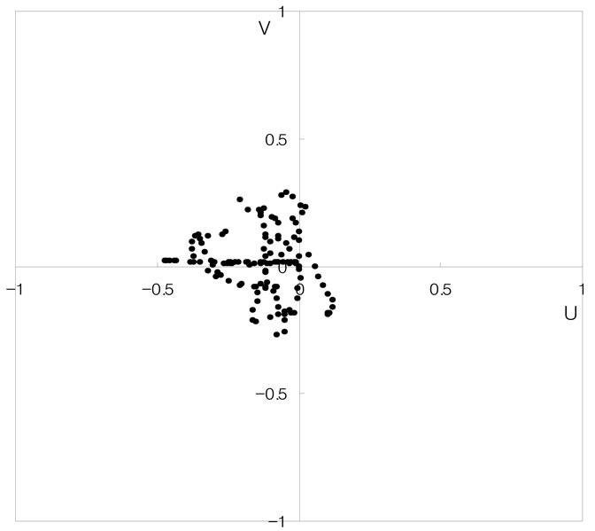
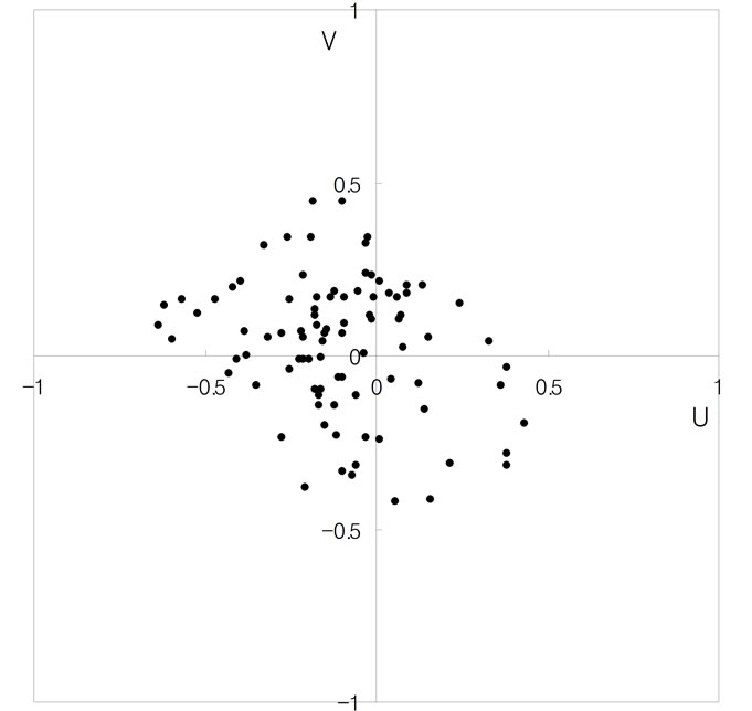
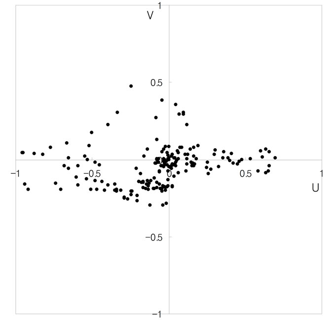
To check the flow characteristics in the groyne area, the flow vector was divided into the vertical direction (U) and the horizontal direction (V) and analyzed using the quadrantmethod. It was marked in the 1st quadrant if the two components of the flow velocity were both positive, and was marked in the 3rd quadrant if both components were negative. An additional review of the LSPIV analysis data against the ADV measurement data was carried out for experiment SF152-90. The maximum flow velocity in the groyne area was discussed in the previous chapter.
For the vertical groyne, the LSPIV analysis data and the ADV measurement data were drawn from the quadrant, as shown in Figures 12 and 13. The overemphasis of the distribution of the flow components in the groyne area on the 2nd and 3rd quadrant is because the core of the vortex was close to the main stream, so that the detection frequency of the flow velocity of the main stream direction was low. Moreover, the reason why this trend is more significant in the LSPIV analysis data is that the number of specimens of the local flow was relatively small because the dropped particles were moved out from the groyne area to the main stream area along the vortex flow. As shown in the figure, as the size of the space of the groynes increased, the distribution of the flow velocity component that circulated along the center was focused on the horizontal axis. Hence, the vertical direction flow velocity component became more dominant compared to the horizontal direction component. This was because as the space of the groynes increased, the shape of the vortex was deformed from a circle shape to an ellipse shape, which was longer in the flow direction (when the space was 4 times longer than the length)
 (a)
(a)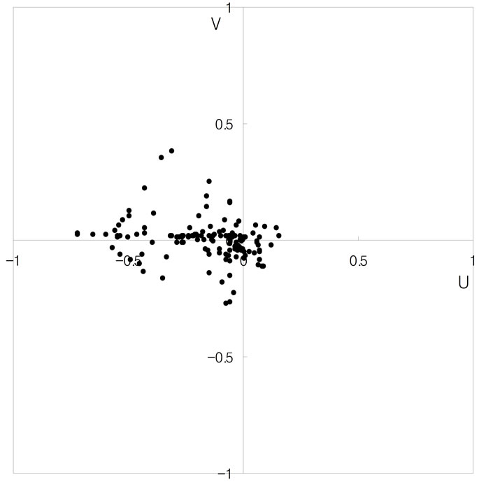 (b)
(b)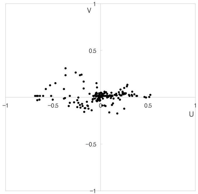 (c)
(c)
Figure 12. Quadrant analysis (SF152/4/6-90, LSPIV). (a) SF152-90; (b) SF154-90; (c) SF156-90.
 (a)
(a)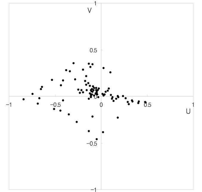 (b)
(b)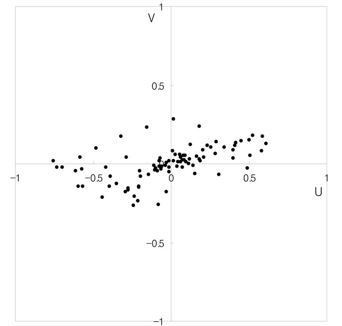 (c)
(c)
Figure 13. Quadrant analysis (SF152/4/6-90, ADV). (a) SF152-90; (b) SF154-90; (c) SF156-90.
or split into two vortexes (when the space was 6 times longer). In the case of the separation, the main vortex was deformed and showed the same trend. In the case of the upstream and downstream groynes, the reverse flow of the main stream appears to be more dominant in the case of the 60˚ upstream groyne (SF204-6) in Figure 14. Moreover, the strong flow velocity in the diagonal direction was measured in the 4th quadrant in the case of the 120˚ downstream groyne (SF152/202-120), which flowed through the downstream geometry of the groyne, showing that it was heading towards the main stream.
The vorticity was calculated from the flow velocity data using the following equation based on the LSPIV method. Since the vorticity indicates the strength of circulation of individual particles, it is not coincident in the whole vortex in the groyne area.
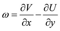 (2)
(2)
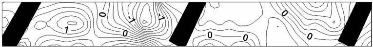
In the above Equation (2), ω U and V indicate the vorticity, the vertical flow velocity component, and the horizontal flow velocity component. When the vorticity had a positive value, it rotated counterclockwise; and when it had a negative value, it rotated clockwise. Figure 15 shows the vorticity contour for the upstream (60˚), the vertical, and the downstream (120˚) groynes. In the case of the 120˚ downstream groyne, there was a strong counterclockwise vorticity at the front part of the first groyne from the upstream groyne, which indicates the strong influence of the scour around the groyne structure.
The maximum value of the vorticity was sequentially bigger along the vertical, upstream, and downstream groynes. For the vertical groyne, the maximum value of the vorticity became bigger along the length of the groyne, but no significant difference appeared when the length of the groyne was bigger than 15% of the width of the channel. The direction of the maximum vorticity is normally clockwise. In the case of the downstream groyne, its value was much bigger than in the cases of the vertical and the upstream groynes by up to 2 - 3 times, and its rotating direction was mostly counterclockwise. It was checked at the strong counterclockwise vortex created at the front part of the 1st groyne at the vorticity contour of the downstream groyne (experiment SF152-120). To survey the change in the mean velocity at the center of the groyne area (except near the bed and the recirculation boundary area) along the length of the groyne, the vertical, upstream (60˚ and 60˚), and downstream (105˚ and 120˚) groynes were prepared without considering the space of the installation. This analysis was made to check the reduction influence against the approaching flow velocity as the basic data for analyzing the influence of aquatics’ habitat.
 (a)
(a)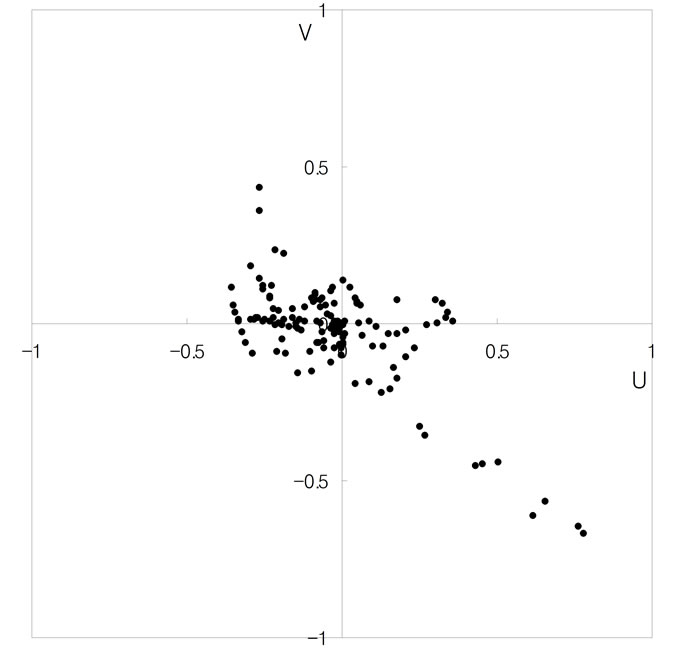 (b)
(b)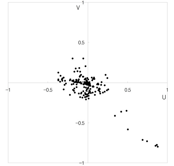 (c)
(c)
Figure 14. Quadrant analysison installed angle. (a) SF204- 60; (b) SF204-120; (c) SF204-120.
 (a)
(a)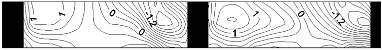 (b)
(b)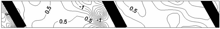 (c)
(c)
Figure 15. Contours of vorticity in groyne flow field: =60, =90, =120, l/B = 0.15, L/l = 2. (a) SF204-60; (b) SF204-120; (c) SF204-120.
5. Conclusions
An irrigating model test was carried out for the space of the groynes in the groyne design factors in this study, and the flow of the groyne area along the space of the groynes was analyzed.
The flow change in the channel area along the space of the groynes seemed to have been influenced by the recirculation zone flow created by the upstream groyne and the flow control along the downstream groyne installation position. When the downstream groyne did not exist, the pattern of the flow in the recirculation area was generated by the groyne downstream stagnant flow and the bank line backward flow. However, the installation of the downstream groyne caused the flow to change because of the change in the stagnant area behind the upstream groyne and the discontinuation of the backward flow at the bank line. Especially, the vortex phenomenon, the most significant flow of the recirculation area, was different from the single groyne and was changed by the space. By virtue of this, one vortex was generated within 31 and two vortexes were generated from 31 to 81. The shape of the vortex changed into an ellipse in the downstream groyne from 81 in the space of the groyne, and three vortexes were generated over 101. The backward flow in the bed area was found to be a very important factor in analyzing the influence of bank erosion. The maximum flow velocity at the bank line was determined to have been around 0.5 of the approaching flow velocity from 41 of the space of the groynes, which had the same value, and was found to have decreased to 50% of the approaching flow velocity from the experimental results. The flow velocity at the bank line was measured at close to zero when the space of the groynes was 1 or 2 times bigger than the length of the groyne. The location of the maximum flow velocity generation differed along the space of the groynes, which seems to be related to the flow change in the groyne area.
From the experiment for the installation angle, 60 experiment cases were carried out for the upstream, vertical, and downstream groynes. Sixty percent of the flow reduction effects showed that the mean flow velocity at the center of the groyne area was reduced by 40% compared to the flow velocity of the inlet from the analysis of the data on the flow velocity. From this result, a shelter for aquatics is possible. The maximum flow velocity in the groyne area sequentially appeared from the upstream, vertical, and downstream groynes. The change in the mean flow velocity in the groyne area along the installation angle and its length showed that the upstream and downstream groynes had more dominant changes in their mean flow velocity than the vertical groyne. From the quadrant analysis of the flow velocity components, the increment and the separation of the vortex in the groyne area was found along the space of the groynes. A strong flow velocity that headed towards the main flow area was measured in the case of the downstream groyne rather than the upstream and vertical groynes, which indicates an active fluid movement in the groyne area. The vorticity indicates the rotation strength of the fluid in the groyne area, which is an important data for the habitat of aquatics. However, a quantitative analysis for vorticity was not performed in this study, and the vorticity of the downstream groyne was found to have been stronger than that of the upstream and vertical groynes in the qualitative analysis along the angle of the installation.
6. Acknowledgements
This study was supported by the Internal Research Project of “River Structure Design Techniques for Harmonizing Nature with the Human” in KICT.
REFERENCES
- A. R. Acheson, “River Control and Drainge in New Zealand, Ministry of Work,” New Zealand, 1968.
- G. B. Fenwick, “State of Knowledge of Channel Stabilization in Major Alluvial River,” Report No. FHWA/ RD-83/099, US Department of Transportation, Washington DC, 1969.
- E. V. Richardson and D. B. Simons, “Spurs and Guide Banks,” Open File Report, Colorado State University Engineering Research Center, Fort Collins, Colorado, 1974.
- P. Jansen, L. Van Bendegorn, J. Van den Berg, M. De Vries and A. Zanen, “Principles of River Engineering,” The Non-Tidal Alluvial River, Pitman, London, 1979.
- B. Z. Kinori and J. Mevorach, “Manual of Surface Drainage Engineering,” Volume II, Streamflow Engineering and Flood Protection, Elsevier, Amsterdam, 1984.
- R. R Copeland, “Bank Protection Techniques Using Spur Dikes,” Miscellaneous paper HL83-1, US Army Engineer Waterways Experiment Station, 1983.
- FHWA, “Design of Spur-Type Streambank Stabilization Structures,” US DOT, FHWA, Rep. No. FHWA/RD 84/101, McLean, 1985.
- R. Ettema and M. Muste, “Scale Effects in Flume Experiments on Flow around a Spur Dike in Flatbed Channel,” Journal of Hydraulic Engineering, Vol. 130, No. 7, 2004, pp. 635-646. doi:10.1061/(ASCE)0733-9429(2004)130:7(635)
- V. Weitbrecht, G. Kuhn and G. H. Jirka, “Large Scale PIV-Measurements at the Surface of Shallow Water Flows,” Flow Measurement and Instrumentation, Vol. 13, No. 5-6, 2002, pp. 237-245. doi:10.1016/S0955-5986(02)00059-6
- J. G. Kang, H. K. Yeo and S. J. Kim, “An Experimental Study on Tip Velocity and Downstream Recirculation Zone of Single Groyne Conditions,” Journal of Korea Water Resource Association, Vol. 38, No. 2, 2005, pp. 143-153. doi:10.3741/JKWRA.2005.38.2.143