Engineering
Vol. 4 No. 4 (2012) , Article ID: 18832 , 5 pages DOI:10.4236/eng.2012.44028
CFD Analysis of Single and Multiphase Flow Characteristics in Elbow*
Mechanical Engineering, University of Michigan-Flint, Flint, USA
Email: qmazumde@umflint.edu
Received January 29, 2012; revised February 23, 2012; accepted March 5, 2012
Keywords: Multiphase Flow; Computational Fluid Dynamics; Elbow; Pressure Drop
ABSTRACT
Computational fluid dynamics (CFD) analysis of singlephase and two-phase flow was performed in a 90 degree horizontal to vertical elbow with 12.7 mm inside diameter. Characteristic flow behavior was investigated at six different upstream and downstream locations of the elbow. To evaluate the effects of different phases, three different air velocities and three different water velocities were used during this study. Commercial CFD code FLUENT was used to perform analysis of both single and multiphase flows. Pressure and velocity profiles at six locations showed an increase in pressure at the elbow geometry with decreasing pressure as fluid leaves from the elbow. Pressure drop behavior observed to be similar for single-phase and multiphase flows. Comparison of CFD results with available empirical models showed reasonably good agreement.
1. Introduction
A phase can be defined as one of the states of matter such as gas or liquid, solid. Multiphase flow is the simultaneous flow of several phases, with two phase flow being the simplest case. The analysis of fluid flow in an elbow is important for a number of engineering applications like heat exchangers, particle transport piping system, air conditioning devices etc. Due to lack of available theory and model for pressure drop calculation in multiphase flow, a computational fluid dynamics study has been performed for single and two phase flow in an elbow and presented in this paper.
Single phase pressure drop for turbulent flow in 90 degree bend was predicted by Crawford [1], using the frictional effects with no available model for separatingflow. Spedding [2] measured the pressure drop in curved pipes and elbow bends for both laminar and turbulent single phase flow and developed empirical correlations. The transitional Reynolds numberfor curved pipesof large bends was also determined using empirical relation. Another model for pressure drop in twophase upward flow in 90 degree bend was proposed by Azzi [3]. In his model the scatter of the logarithmic ratios of the experimental and the predicted values amounts to about 25% and is substantially lower than that observed with selected models recommended in the literature. This model included physically consistent the usual design parameters and the limits of single-phase gas as well as liquid flow.
Detailed studies of two-phase pressure drop have largely been confined to the horizontal plane. Chenoweth and Martin [4] showed that while two phase pressure drop around bends was higher compared to single-phase flow it could be correlated by adoption of the LockhartMartinelli [5] model developed originally for straight pipe. Chisholm [6] presented another model for prediction of two phase pressure drop in bends, based on Φ2LA, for all pipe diameters, bend radius ratios (R/d) and different flow rates. Shannak Benbella [7] reported that total pressure drops in internally wavy pipe bends are approximately 2 - 5 times higher than those in smooth bends.
The main variables which characterize two phase flow are the increased pressure drop that occurs when a liquid is introduced into a tube with gas flow and the fractional pipe volume occupied by the flowing liquid. These two parameters are the minimum information needed for design of piping systems where two phases flow simultaneously. Liquid entrainment and flow patterns are also important variable in two phase flow phenomena. The problem of liquid phase residence time distribution in two phase flow has not received much attention as in single phase pipe flow. However, the importance of such information for fluid contactors and reactors is generally recognized [8].
Turbulent shear flow in curved duct was investigated by Ellis [9] comparing the result of two curved rectangular flow with a straight duct flow. Mean velocity profiles, turbulence intensity distributions and stream wise energy were presented for turbulent air flow in a smooth-walled duct by Hunt [10]. The study was conducted in high aspect ratio rectangular duct with small stream wise curvature, and was compared with measurements taken in a similar straight duct. Humphrey [11] investigated the steady, incompressible, isothermal, developing flow in a square-section curved duct with smooth walls. The longitudinal and radial components of mean velocity and corresponding components of the Reynolds stress tensor were measured with a laser-Doppler anemometer along with the secondary mean velocities, driven mainly by the pressure field. Turbulent flow in 90˚ square duct and pipe bends was numerically computed by Briley [12] using Navier-Stokes equation. The numerical solution of the compressible Reynolds averaged Navier-Stokes equations in the low Mach number regime (M = 0.05) was used to approximate the flow of liquid.
2. The CFD Modeling
With the advancement and recent development of CFD codes, a full set of fluid dynamic and multiphase flow equations can be solved numerically. The current study used commercial CFD code, FLUENT [13], to solve the balance equation set via domain discretization, using control volume approach. These equations are solved by converting the complex partial differential equations into simple algebraic equations.
Three dimensional unstructured mesh was used in this study for the pipe and elbow sections using an implicit method for solving the mass, momentum, and energy equations. The mixture composition and phase velocities were defined at the inlet boundary of the pipe upstream of the elbow. The к-ε turbulence model with standard wall functions were used due to their proven accuracies in solving mixture problems. The gravitational acceleration of 9.81 m/s2 in upward flow direction was used.
2.1. Geometry Details
CFD simulation was performed to investigate pressure drop and velocity profiles of single and two-phase flows in a 12.7 mm inside diameter, 90 degree elbow with an r/D ratio of 1.5. The r/D ratio of 1.5 was used, as this represents a standard elbow configuration commonly used in industrial applications. Analysis results at six different locations upstream and downstream of the elbow were used in this study as shown in Figure 1. The distance between each location in the straight pipe sections was 50.8 mm or four times the pipe diameter. A combination of hexahedral cell edge mapping mesh scheme available in GAMBIT has been selected for the face mesh generation. This mesh was then swept along an edge to create
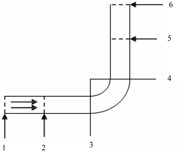
Figure 1. Elbow geometry with straight pipe sections.
the entire volume of flow. With a greater number of mesh elements, convergence problems were encountered in this simulation. A mesh sensitivity analysis was performed that enabled the optimization of the mesh size in the radial and axial direction of the elbow.
Hexahedral mesh was used due to its capabilities in providing high-quality solution with fewer numbers of cells than comparable tetrahedral mesh for simple geometry. The meshed elbow geometry with inlet flow domain is shown in Figure 2. The total number of nodes in the model was 118,110 with 333,402 faces and 108,790 cells. After modeling the flow domain, grid generation is a key issue in flow simulation that governs the stability and the accuracy of the predictions. A very fine grid is computationally more expensive, and is necessary to ensure reasonable resolution of the mesh. The flow field in the vicinity of the wall has steep velocity gradients; hence finer grid is desirable in this region.
2.2. Multi Phase Modeling
In the present study the mixture model approach was used where different phases are treated mathematically as interpenetrating continua and the concept of phase volume concentrations were assumed to be continuous functions of space and time. Mixture model is relatively easy to understand and accurate for multi-phase flow analysis compared to Eulerian and VOF (Volume of Fluid) models.
The mixture model is a simplified multiphase model that can be used for flows where the phases move at different velocities. The mixture model is also capable to model any number of phases (fluid or particulate) by solving the momentum, continuity, and energy equations for the mixture, the volume fraction equations for the secondary phases, and algebraic expressions for the relative velocities. The mixture model is a good substitute of the Eulerian multiphase model as full multiphase model may not be feasible when there is a wide distribution of phases or when the inter-phase laws are unknown or
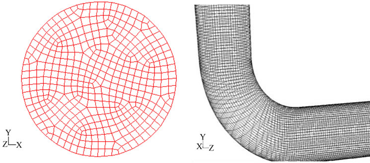
Figure 2. Meshed elbow geometry and inlet flowdomain.
their reliability can be questioned. The mixture model can perform similar to other full multiphase model while solving a smaller number of variables using a single-fluid approach and allowing the phases to be interpenetrating. The volume fractions of gas and liquid phases, αG and αL for a control volume can be any value between 0 and 1. It also allows the phases to move at different velocities, using the concept of slip velocities. When the phases are move at the same velocity, the mixture model is reduced to homogeneous multiphase model.
2.3. Modeling Assumption
In addition to the models and parameters discussed previously, other assumptions involved in the CFD simulations are stated below. In addition to steady state flow, the effect of temperature change on the flow has been neglected assuming isothermal conditions. Due to relative simplicity of the flow geometry, absence of strong body forces and relatively high flow rates, standard wall functions have been selected and are assumed to effectively model the near-wall viscosity affected regions for the turbulent flows. Since the continuous phases considered in the present study are all liquids, no slip boundary conditions are assumed at the wall of tubing. The effect of wall roughness on the flow and shear stress has not been investigated.
3. Solution Strategy and Convergence
A calculation of multiphase flow for a complex geometry such as elbow requires an appropriate numerical strategy to avoid a divergent solution. Instead of using a steadystate solution strategy, the use of a transient solution with quite small time steps gives convergent solutions and reasonable results. A second order upwind discretization scheme was used for the momentum equation while a first order upwind discretization was used for the volume fraction, energy, turbulence kinetic energy and turbulence dissipation rate. These schemes ensured, in general, satisfactory accuracy, stability and convergence. The convergence criterion is based on the residual value of the calculated variables, i.e., mass, velocity components, energy, turbulence kinetic energy, turbulence dissipation rate and volume fraction. In the present calculations, the threshold values were set to a ten thousandth of the initial residual value of each variable, except the residual value of energy which was a millionth. The residual value of energy requires a very small value to ensure accuracy of the solution. In pressure-velocity coupling, the phasecoupled SIMPLE algorithm [14] was used as an extension of the SIMPLE algorithm [15] to multiphase flows. Other solution strategies used were the reduction of under relaxation factors of momentum, the volume fraction, the turbulence kinetic energy and the turbulence dissipation rate to bring the non-linear equation close to the linear equation.
4. CFD Analysis and Results
Analyses were performed for nine different combinations of air and water velocities as shown in Table 1. The air velocities were increased by factors of 2 and 3; the water velocities were increased by a factor of 10 from the initial condition.
The CFD analysis results are presented as cross-sectional pressure and velocity profiles. Figure 4 shows the pressure at locations 2, 3, 4 and 5 of the el-bow as defined in Figure 1. The first column of Figure 4 presents contours for single phase air with 15.24 m/sec; the second column is for single-phase water with 0.1 m/sec velocity. The third column shows the pressure and velocity contours for multiphase flow with corresponding air and water velocities. The top of each individual contour diagram represents the inner wall of the elbow and the bottom part of the contour represents the outer wall of the elbow. For single-phase water velocity of 0.1 m/sec, higher pressure was observed at the wall forming a high pressure thin annular pattern. For single-phase air and multiphase air-water flows, the pressure distribution at location 2 is dispersed without forming any regular pattern. At locations 3 and 4 higher pressures observed at the inner wall with lower pressure at the outer wall of the elbow that reversed as the flow progressed to location 5 at downstream straight pip section of the elbow.
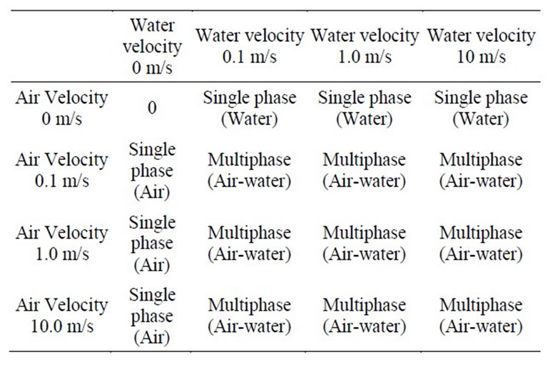
Table 1. Air-water velocities used in CFD analysis.
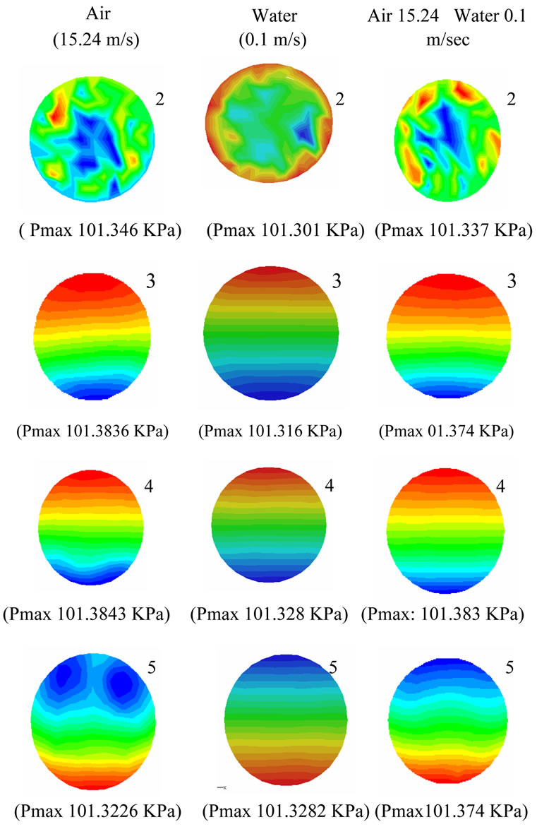
Figure 4. Pressure drop at different location in elbow for single and multiphase flows.
Figures 5-6 shows the pressure distributions profiles at location 1 - 5 in the elbow geometry for single phase and multiphase air-water flows. It appears that pressure de-creases between location 1 and 2 for multiphase airwater flow and increases back in locations 3 and 4 as flow enter the elbow section and then decreases when the flow exits the elbow to straight pipe section. For single phase air or water flows, a continuous increase in pressure is observed between locations 1 and 4 and with pressure decreasing between locations 4 and 5.
5. Validation of CFD Results with Empirical Models
To predict pressure drop in elbows for single and multiphase flows a number of empirical models have been evaluated [16-19]. These models can be classified into four basic groups: homogeneous model, separated flow model, dimensional and similitude approach and Chisholm approach. All these models use global approaches because they do not make any reference to a specific flow pattern presented in the elbow. These approaches,
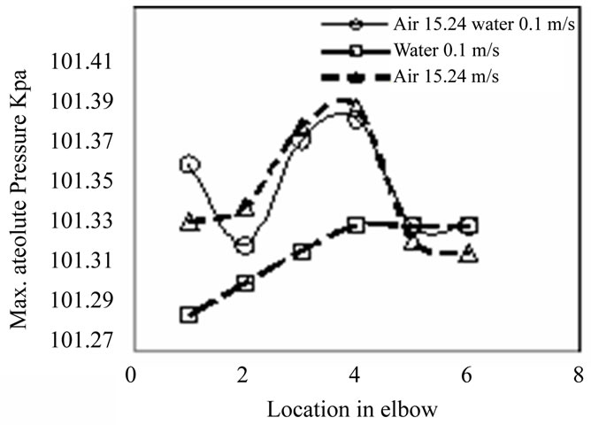
Figure 5. Single and multiphase pressure drop for Air = 15.24 m/sec, Water = 0.1 m/sec
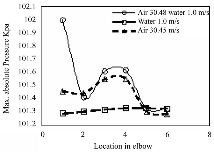
Figure 6. Single and multiphase pressure drop for Air = 30.48 m/sec, Water = 1.0 m/sec.
with the exception of the homogeneous model, were developed using experimental data provided by several authors [20].
Pressure drop calculations were performed using the abovementioned empirical models for similar flow conditions. Due to unknown variables and complexities associated with calculations with Dukler and Martinelli models, the results obtained were not reliable. However, Chisholm model and Benbella models provided reliable results for a wider range of conditions. Chisholm model was adjusted by a dimensionless relationship which is a function of the homogeneous volumetric function and dean number [21].
Pressure drop results of CFD analysis, Chisholm model and Benbella Model are presented in Table 2. For low water velocity of 0.1 m/sec, Chisholm model predicted pressure drops were higher than both CFD and Churchill model predictions. At 1.0 m/sec water velocity, Benbella model predicted higher pressure drop compared to Chisholm model with even higher predictions in CFD results. At 10.0 m/sec water velocity, and 15.4 m/sec air velocity, Benbella model predicted highest pressure drop. However for the same water velocity, with 45.72 m/sec
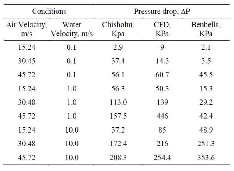
Table 2. Comparison of CFD and empirical model predicted pressure drops (Kpa) [7,18].
air velocity, CFD predicted pressure drop value was 2 times higher than Chisholm and lower than Benbella model predictions.
6. Summary and Conclusion
CFD analysis of single and two phase flow in a 12.7 mm elbow was performed using FLUENT. Analysis performed for three different air velocities between 15.24 - 45.72 m/sec and three different water velocities of 0.1 to 10.0 m/sec. Pressure drop profiles and cross-sectional pressure contour maps were presented for characteristic flow behaviors in both single and multi-phase flows. CFD results were compared with two different empirical models showing reasonable agreement.
REFERENCES
- N. M. Crawford, G. Cunningham and P. L. Spedding, “Prediction of Pressure Drop for Turbulent Fluid Flow in 90˚ Bends,” Proceedings of the Institution of Mechanical Engineers, Vol. 217, No. 3, 2003, pp. 153-155. doi:10.1243/095440803322328827
- P. L. Spedding, E. Benard and G. M. McNally, “Fluid Flow through 90˚ Bends,” Developments in Chemical Engineering and Mineral Processing, Vol. 12, No. 1-2, 2004, pp. 107-128. doi:10.1002/apj.5500120109
- A. Azzi and L. Friedel, “Two-Phase upward Flow 90˚ Bend Pressure Loss Model,” Forschung im Ingenieurwesen, Vol. 69, No. 2, 2005, pp. 120-130. doi:10.1007/s10010-004-0147-6
- J. M. Chenoweth and M. W. Martin, “Turbulent TwoPhase Flow,” Petroleum Refiner, Vol. 34, No. 10, 1955, pp. 151-155.
- R. W. Lockhart and R. C. Martinelli, “Proposed Correlation of Data for Isothermal Two-Phase Two-Component Flow in Pipes,” Chemical Engineering Progress, Vol. 45, No. 1, 1949, pp. 39-48
- D. Chisholm, “Two-Phase Flow in Pipe Lines and Heat Exchangers,” Journal of Heat Transfer, Vol. 129, 1983, pp. 101-107.
- S. Benbella, M. Al-Shannag and Z. A. Al-Anber, “GasLiquid Pressure Drop in Vertical Internally Wavy 90 Degree Bend,” Experimental Thermal and Fluid Science, Vol. 33, No. 2, 2009, pp. 340-347. doi:10.1016/j.expthermflusci.2008.10.004
- G. R. Rippel, C. M. Eidt Jr. and H. B. Jordan, “Two Phase Flow in a Coiled Tube, Pressure Drop, Holdup, and Liquid Phase Axial Mixing,” Industry & Engineering Chemistry Process Design and Development, Vol. 5, No. 1, 1966, pp. 32-39. doi:10.1021/i260017a007
- L. B. Ellis and P. N. Joubert, “Turbulent Shear Flow in a Curved Duct,” Journal of Fluid Mechanics, Vol. 62, No. 1, 1974, pp. 65-84. doi:10.1017/S0022112074000589
- I. A. Hunt and P. N. Joubert, “Effects of Small Streamline Curvature on Turbulent Duct Flow,” Journal of Fluid Mechanics, Vol. 91, No. 4, 1979, pp. 633-659. doi:10.1017/S0022112079000380
- J. A. C. Humphrey, J. H. Whitelaw and G. Yee, “Turbulent Flow in a Square Duct with Strong Curvature,” Journal of Fluid Mechanics, Vol. 103, 1981, pp. 443-446. doi:10.1017/S0022112081001419
- W. R. Briley, R. C. Buggeln and H. McDonald, “Computational of Laminar and Turbulent Flow in 90˚ SquareDuct and Pipe Bends Using the Navier-Stokes Equations,” DTIC Report No. R82-920009-F, 1982.
- I. Fluent, “Fluent 6.3 User Guide,” Fluent Inc., Lebanon, 2002.
- S. A. Vasquez and V. A. Ivanov, “A Phase Coupled Method for Solving Multiphase Problem on Unstructured Meshes,” Fluids Engineering Division Summer Meeting, ASME, Boston, 11-15 June 2000.
- S. V. Patankar, “Numerical Heat Transfer and Fluid Flow,” McGraw-Hill, New York, 1980.
- R. W. Lockhart and R. C. Martinelli, “Proposed Correlation of Data for Isothermal Two-Phase Two-Component Flow in Pipes,” Chemical Engineering Progress, Vol. 45, No. 1, 1949, pp. 39-48.
- A. E. Dukler, M. Wicks III and R. G. Cleveland, “Frictional Pressure Drop in Two-Phase Flow B. An Approach through Similarity Analysis,” AIChE Journal, Vol. 10, No. 1, 1964, pp. 44-51. doi:10.1002/aic.690100118
- D. Chisholm, “Two-Phase Flow in Pipe Lines and Heat Exchanges,” Pitman Press, Ltd., Longman Higher Education, USA, 1983.
- G. B. Wallis, “One Dimensional Two-Phase Flow,” McGraw-Hill, New York, 1969.
- G. Hetsroni, (Ed.), “Handbook of Multiphase Systems,” Hemisphere McGraw Hill, New York, 1982.
- S. F. Sánchez, R. J. C. Luna, M. I. Carvajal and E. Tolentino, “Pressure Drop Models Evaluation for Two-Phase Flow in 90 Degree Horizontal Elbows,” Ingenieria Mecanica Techilogia y Desarrollo, Vol. 3, No. 4, 2010, pp. 115-122.
NOTES
*CFD Analysis of Single and Multiphase Flow Characteristics in Elbow.