Engineering
Vol. 3 No. 6 (2011) , Article ID: 5339 , 8 pages DOI:10.4236/eng.2011.36071
The Effects of Dimension Ratio and Horizon Length in the Micropolar Peridynamic Model
Aeronautical Engineering Department, Faculty of Aeronautics and Astronautics, Istanbul Technical University, Istanbul, Turkey
E-mail: ozkol@itu.edu.tr
Received January 6, 2011; revised May 16, 2011; accepted May 25, 2011
Keywords: Peridynamics, Micropolar Peridynamics, Non-local continuum mechanics, Horizon
ABSTRACT
The aim of this study is to investigate the effects of horizon selection on the elastic behaviour of plate type structures in the micropolar peridynamic theory. Plates with various lengths and widths have been investigated using micropolar peridynamic model for different horizon selections. The mathematical model of plates has been provided applying the micropolar peridynamic theory and solution of this model has been obtained by finite element methods. The displacement fields have been computed for the different horizons and dimension ratios of plates. To compute the displacement field a program code has been developed by using the software package MATHEMATICA. The results obtained have been compared with the analytical solution of the classical elasticity theory and with the solution of displacement based finite element methods. For displacement based finite element method solution the software package ANSYS has been used. According to results it has been observed that the displacement fields of the plates are strongly affected by horizon selection. Therefore a question raises that which horizon length should be used with the problem in hand or is there any method to find the appropriate/best horizon length.
1. Introduction
In classical theory of continuum mechanics, a representative volume element of the material is chosen then reaction of this material to homogeneous deformation is described as stress and strain relation. Formulation of stress and strain depends on deformation gradients and their derivatives. From mathematical aspect when there is a discontinuity, such as crack or phase boundary, the deformation gradients and their derivatives can not be calculated. The discontinuous area is reformulated in order to solve the problem in classical theory. But recovering approaches depend on the severity of the problem and these are unique solutions for the problem. For example, “crack tips are considered body surfaces with particular boundary conditions. Crack tips satisfy a particular energy balance that is different from the rest of the body. Phase boundaries are surfaces inside the body that satisfy particular jump conditions and kinetic relations” [1].
To provide a solution, Silling has purposed a new theory called peridynamic [2]. The theory uses integral equation instead of spatial derivatives of displacement. This feature of the theory makes it valid on continuous and discontinuous areas. Since the particles interact with each other with a finite distance, the theory is categorized as non-local model. In the peridynamic theory the particles, only inside the horizon, interact with each other and the force between particles is expressed with vector valued function  as shown in Figure 1.
In the past using Pridynamic theory, impact of a sphere on a brittle target [3], dynamic growth of a single crack from a defect in membranes and bursting of a balloon have been illustrated [4]. In addition, analysing an infinite bar under self-equilibrated load with peridynamic theory, it has been observed that there is decaying displacement propagation different than classical results and it has been showed that, taking the horizon zero the theory is converges to classical continuum theory [5]. Also for different fracture conditions initial value problems has been solved [6,7].
The wave propagation in anisotropy condition has been analyzed [8]. The force flux and peridy-namic stress have been defined representing the peridynamic state and
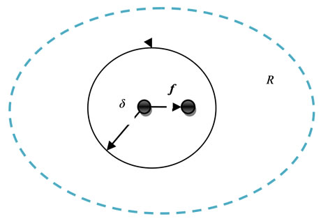
Figure 1. The material horizon and pairwise force function.
constitutive equations [9-11]. These definitions have been implemented using finite element method [12]. The conditions in which peridynamic theory converges to classical theory have been showed using pridynamic stress definition [13].
The implementation of peridynamic theory with molecular dynamic code has been carried out and the similarities have been emphasized [14]. Recently, for composites progressive damage prediction and error prediction for brittle materials such as glasses have been studied [15]. Also using peridynamic theory, the material stability and and failure analysis have been carried out [16].
However, the most important shortcoming of the peridynamic theory is the Poisson`s ratio limitation. The theory is applicable to material only with Poisson’s ratio 1/4 Therefore a few years later, including peridynamic moment in addition to central forces, Gerstle, Sau and Silling proposed the micropolar peridynamic theory as a generalization of the peridynamic theory. Furthermore, it is possible to use the micropolar theory in the finite element method with harmony. This gives easy application of boundary conditions to physical model in hand [17].
Although various applications of peridymanic and microplolar peridynamic model have been done as seen from the literature, the effect of dimension ratio or horizon selection has not been analyzed so far. The main objective of this work is to investigate these fundamental features.
2. Fundamental Definition of Peridynamic and Micropolar Peridynamic Theory
2.1. Peridynamic Theory
In peridynamic theory, inside the horizon length particles interact with each other with a central vector valued  function. The parameters of
  functions are displacement vectors and position vectors.
  is zero if the particles are not inside the horizon. The integration of
  function over a unit volume is a force function such as
 ![]() in the unit of force per reference volume [2].
in the unit of force per reference volume [2].
According to these definitions the quantity of force function![]() , at any time t and at any point x in the reference configuration, is described as follows,
, at any time t and at any point x in the reference configuration, is described as follows,
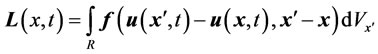 (1)
(1)
By applying the the Newton’s Second Law, the peridynamic equation of motion can be written as follows:
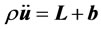 (2)
(2)
where
 is prescribed loading force density in the unit of per-unit reference volume.
In order to simplify the writing of the equation, some notations are described as ,
,  and
and .
.
Then, relative displacement vector:
 (3)
(3)
And relative position vector:
 (4)
(4)
Now the relative position of the particle in the deformed configuration:
 (5)
(5)
When  the equation (2) is described as equilibrated.
Other basic restrictions for f are linear admissibility condition and angular admissibility condition. According to Newton’s Third Law the common force between two particles has same magnitude but opposite direction. Therefore the forces must have opposite signs.
 (6)
(6)
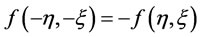
This condition is called linear admissibility. Also the force between particles must be in the direction of their relative current position.
 (7)
(7)
This condition is called angular admissibility.
2.2. Micropolar Peridynamic Theory
In the micropolar peridynamic model, besides peridynamic central forces, the peridynamic moments are also considered, and particles interact with each other inside the material horizon. Infinitesimally-small particle i and j interact with each other over a finite distance in the domain R. The horizon definition is same as in section 2.1 [17].
The total force in unit volume  acting on the particle i by the particle j is written as [18],
where,
 The pairwise force vector between particle
  and
and  defined in terms of force per unit reference volume squared.
 Unit volume of particle j
The total moment in unit volume  acting on particle i by particle j is written as below.
 (9)
(9)
where,
 The pairwise moment vector between particle
  and
and  presented in terms of moment per unit reference volume squared.
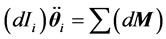
According to Newton’s Second Law conservation of linear momentum is given by:
 (10)
(10)
And the conservation of angular momentum is:
 , (11)
where,
 : Force vector acting on body
 : Moment vector acting on body
 : Differential mass of particle i
 : Differential mass moment of inertia of the particle i
 Acceleration of the particle i
![]() Angular acceleration of particle i For static condition the equations takes the following forms;
Angular acceleration of particle i For static condition the equations takes the following forms;
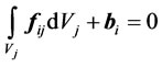 (12)
(12)
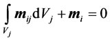 (13)
(13)
where,
![]() Vector valued external force defined in terms of force per unit reference volume.
Vector valued external force defined in terms of force per unit reference volume.
 Vector valued external moment defined in terms of moment per unit reference volume.
When the material is homogeneous and elastic, the variables of  and
and  functions are relative displacement, relative position of the particles initially, and rotations of the particles.
3. Finite Element Approach of Micropolar Peridynamic Theory
In peridynamic theory, the bond between two particles could be thought as micro truss, there is only axial tension or compression. But in micropolar peridynamic theory the bond is micro beam. Therefore, bending and torsion features can be added [17].
Due to benefits of Finite Element Method such as easy application of boundary condition and efficient computation, Gerstle, Sau and Silling implemented the FEM to the micropolar theory. A micropolar peridynamic frame element has been used to derive the finite element formulation of the theory [17]. The frame element has radially simetric cross sectional area A, it’s bending moment of inertia is I and torsional moment of inertia is 2I and length of the frame element is L as shown in the Figure 2.
Young’s modulus of the element is . c, d and
 ![]() are three independent material parameter.
are three independent material parameter. ![]() represents horizon, c and d are the elastic properties of the element where,
represents horizon, c and d are the elastic properties of the element where,
 (14)
(14)
 (15)
(15)
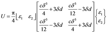
In terms of c and d the stiffness matrix of a peridynamic frame element  is shown as below,
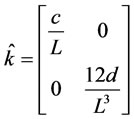 (16)
(16)
Differential force on particle i and j and differential elastic strain energy in the particle i and j are given as follows,
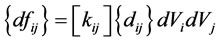 (17)
(17)
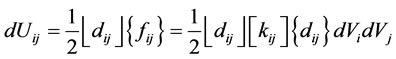 (18)
(18)
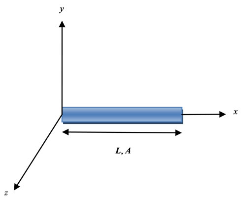
Figure 2. Features of the peridynamic element.
where, stiffness matrix k is in global coordinates while stiffness matrix  is in local coordinates according to position of the frame element.
Total strain energy of the body is expressed as,
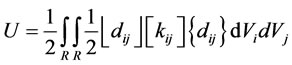 (19)
(19)
In a more convenient form, to apply numerical solution technique, equation (19) can be written in the following form:
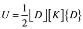 (20)
(20)
where, D is nodal displacements and K is stiffness matrix of the body.
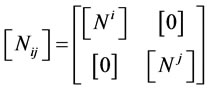
For easy application global stiffness matrix can be written as below by separating as contribution of particles in the same element and contribution of the particles in the different elements.
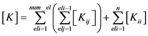 (21)
(21)
 and
and  matrices are given by:
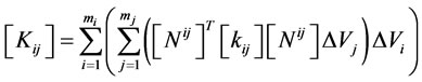 (22)
(22)
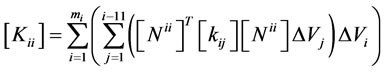 (23)
(23)
Shape matrices  and
and  can be expressed as follows:
 (24)
(24)
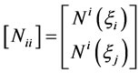 (25)
(25)
While comparing the stored energy in the unit volume, i.e. strain energy, parameters of the classical theory and the parameters of the micropolar peridynamic theory can be related to each other. The parameters of the classical theory are Modulus of Elasticity E and Poisson’s Ratio![]() , the strain energy is calculated in terms of these parameters. The micropolar peridynamic theory calculates the strain energy in terms of c and d.
, the strain energy is calculated in terms of these parameters. The micropolar peridynamic theory calculates the strain energy in terms of c and d.
For two-dimensional plane stress condition assuming uniform strain field, the energy density of unit volume body using principle strains has the following matrix form in classical theory:
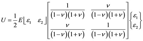 (26)
(26)
The strain energy in the material horizon for a unit volume in the case of applying micropolar peridynamic theory is expressed as below:
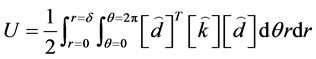 (27)
(27)
 (28)
(28)
To relate c and d to E and ![]() the equations (26) and (28) are compared, and c and d have been written in terms of E,
the equations (26) and (28) are compared, and c and d have been written in terms of E, ![]() and
and ![]() as follow,
as follow,
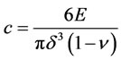 (29)
(29)
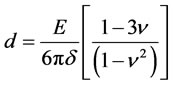 (30)
(30)
Choosing appropriate E, ![]() and
and ![]() the structure can be modeled using micropolar peridynamic theory.
the structure can be modeled using micropolar peridynamic theory.
4. Application of Micropolar Peridynamic Theory
In order to carry out the analysis on cantilever plates by applying micropolar peridynamic model a computer code has been developed using software package MATHEMATICA.
E, ![]() ,
, ![]() , a (length), b (width), t (thickness), p (particle number in one element), boundary conditi-ons and Q (force applied externally) are input parameters for the program code while K and D are output parameters.
, a (length), b (width), t (thickness), p (particle number in one element), boundary conditi-ons and Q (force applied externally) are input parameters for the program code while K and D are output parameters.
Seven cantilever plates with various length and width have been analyzed for four different horizon selections using developed code. Material selected is Aluminum 1100 H12 which has material properties as E = 70000 Mpa and v = 0.33 [19]. 500N concentrated external load has been applied to free end in the –y direction. Thickness for all models is constant as 1 mm. The ratios of length to width are chosen from 1 to 7 as seen in Table 1 and in Table 2 horizon selections for each model is shown.
For analytical result the equation (31) for elastic plates is used and the model for the equation is as in Figure 3 [20].
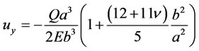 (31)
(31)
For numerical solution displacement-based finite element model analysis is carried out using software package ANSYS.
5. Results
The maximum displacements are obtained using Micropolar Peridynamic (MPD) for four different horizon
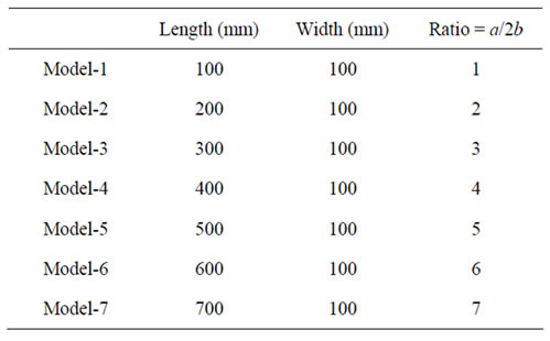
Table 1. Dimensions of the samples.
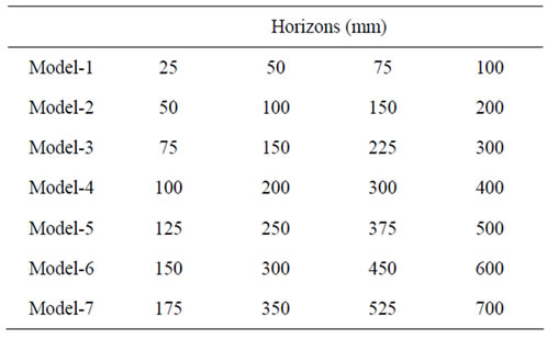
Table 2. Horizon selection of models.
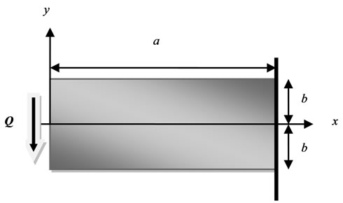
Figure 3. Cantilever plate with an end load.
selections for each model, classical-analytical approach and ANSYS. Results for each model are shown graphically.
Table 3 shows the maximum displacements of models according to ANSYS and classical-analytical results and Table 4 shows the maximum displacements of each model for four different horizon selections.
While in each figure continuous curve represents MPD results, the symbols square and triangle show the Classical and ANSYS results respectively.
The continuous curves are obtained and shown in figures 4-10 for various horizon selections, however Classical theory and ANSYS results do not depend on the horizon.
By close inspection of figures reveals out that, maximum displacements strongly depend on the horizon se-
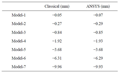
Table 3. Maximum displacements of Classical and ANSYS results.
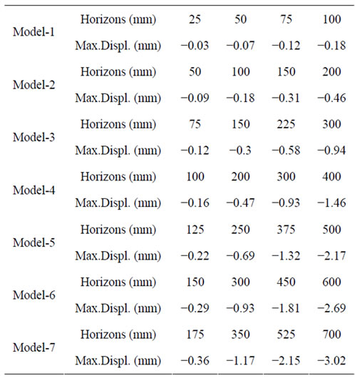
Table 4. Maximum displacements of MPD for various horizons.
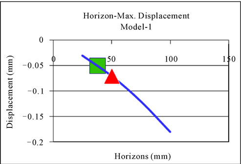
Figure 4. Maximum displacements versus horizons for Model-1.
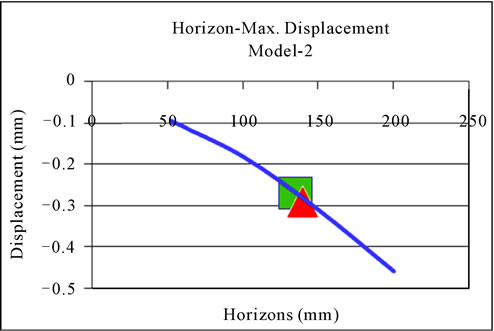
Figure 5. Maximum displacements versus horizons for Model-2.
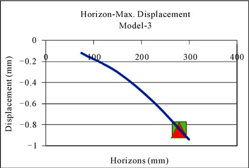
Figure 6. Maximum displacements versus horizons for Model-3.
lection. For the first three models, for some certain horizon selection, there are points at which classical and ANSYS results coincide. However, for the models dimension ratios are bigger than three, the results of classical theory do not coincide with the results of MPD for
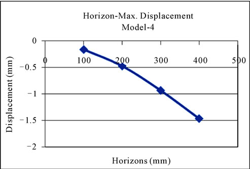
Figure 7. Maximum displacements versus horizons for Model-4.
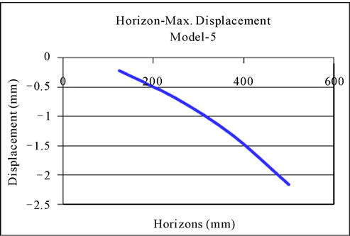
Figure 8. Maximum displacements versus horizons for Model-5.
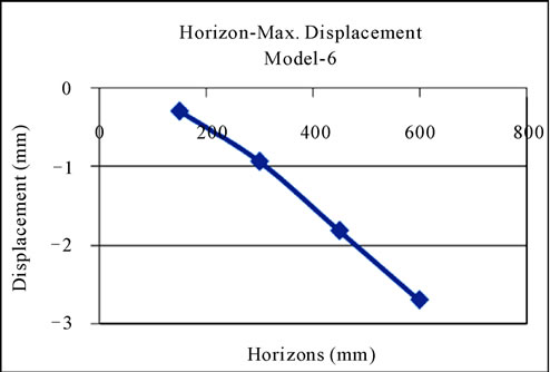
Figure 9. Maximum displacements versus horizons for Model-6.
any horizon selection. Since, the most accurate value should be obtained when horizon length includes every point in a body, maximum displacement of the seven models according to MPD, classical-analytical and ANSYS results have been compared. Additionally, the errors
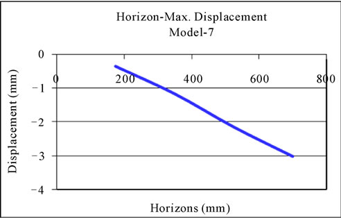
Figure 10. Maximum displacements versus horizons for Model-7.
between MPD and ANSYS results, MPD and classicalanalytical results have been calculated and shown in the Figures below.
Figure 11 shows maximum displacements calculated by using Micropolar Peridynamic theory, ANSYS and classical-analytical theory. Figure 12 and Figure 13 show the error with respect to the results obtained by using the classical theory and ANSYS, respectively.
In Model-3 the error takes its minimum value for both analytical solutions and ANSYS results but then the error increases for both results. The graphical representation of error for maximum displacement shows increasing trend.
6. Conclusion and Discussion
In this study MPD, classical-analytical and ANSYS analysis of seven the plates with various length and width have been carried out. Each plate has been analyzed for four different horizon selections. It has been observed from tables 3 and 4 that the displacement fields of plates obtained by MPD are strongly affected by horizon selections. In model-1, model-2 and model-3 for some horizon selection the MPD gives the same results with Classical and ANSYS solutions. However, for other models, the results for the maximum displacements never have the same values. The concept of horizon is the most important difference between classical and Peridynamic model. So it is significant that there is a generalized rule to choose the appropriate horizon length.
Also physically one expects that the most accurate solution must be obtained when the horizon is selected as it contains all points of the body. When one compares that case with analytical and ANSYS result, it can be seen from Figure 11 that, in MPD, the model underestimates the displacement which can be translated as MPD illustrates the model more rigid than it is.
In addition, it is shown from Figure 11 that the displacement fields of the plates are strongly affected by
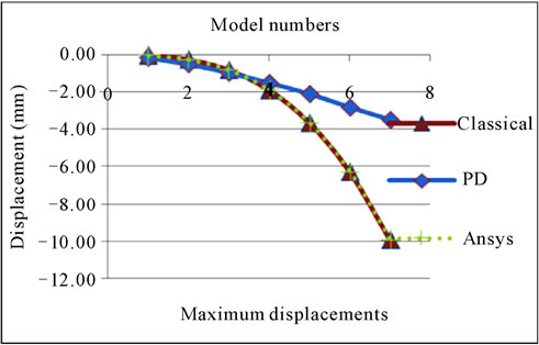
Figure 11. Maximum displacements.
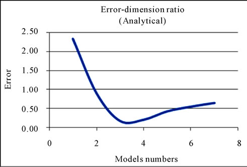
Figure 12. Error with respect the results using the classical theory.

Figure 13. Error with respect to the results from Ansys.
dimensional changes of the plates. This shows that The MPD might have a shortcoming of validity on every dimension ratios and horizon selection. Even if appropriate horizon could be found for some dimension ratios, there would be no explanation about which horizon could be selected.
Apparently, there is a problem which is related both to dimension ratios and horizon length selection. This might be solved by checking the mathematical model and physical basis on which the theory has been developed.
7. REFERENCES
- M. Zimmerman, “A Continuum Theory with Long-Range Forces for Solids,” Ph.D. Thesis, Massachusetts Institute of Technology, Boston, 2005.
- S. A. Silling, “Reformulation of Elasticticity Theory for Discontinuities and Long Range Forces,” Journal of the Mechanics and Physics of Solids, Vol. 48, No. 1, 2000, pp. 175-209. doi:10.1016/S0022-5096(99)00029-0
- S. A. Silling and E. Askari, “A Meshfree Method Based on the Peridynamic Model of Solid Mechanics,” Journal of Computers and Structures, Vol. 83, No. 17-18, June 2005, pp. 1526-1535.
- S. A. Silling and F. Bobaru, “Peridynamic Modeling of Membranes and Fibers,” International Journal of NonLinear Mechanics, Vol. 40, 2005, pp. 395-409. doi:10.1016/j.ijnonlinmec.2004.08.004
- S. A. Silling, M. Zimmerman and R. Abeyaratne, “Deformation of a Peridynamic Bar,” Journal of Elasticity, Vol. 73, No. 1-3, 2003, pp. 173-190. doi:10.1023/B:ELAS.0000029931.03844.4f
- S. A. Silling, “Peridynamic Modeling of the Failure of the Heterogeneous Solids,” 2002. http://www.sandia.gov/emu/aro-vg.pdf
- E. Emmrich and O. Weckner, “Analysis and Numerical Approximation of an Integro Diff. Equ. Modeling Non_Local effects in linear elasticity,” Mathematics and Mechanics of Solids, Vol. 12, No. 4, 2005, pp. 363-384. doi:10.1177/1081286505059748
- A. Chakraborty, “Wave Propagation in Anisotropic Media with Non-Local Elasticity,” International Journal of Solids and Structures, Vol. 44, No. 17, August 2007, pp. 5723- 5741. doi:10.1016/j.ijsolstr.2007.01.024
- S. A. Silling, M. Epton, O. Weckner, C. Xu and E. Askari, “Peridynamic States and Constitutive Modeling,” Journal of Elasticity, Vol. 88, No. 2, 2007, pp. 151-184. doi:10.1007/s10659-007-9125-1
- R. B. Lehoucq and S. A. Silling, “Force Flux and the Peridynamic Stress Tensor,” Composite Structures, Vol. 56, No. 4, April 2008, pp. 1566-1577.
- T. L. Warren, S. A. Silling, A. Askari, O. Weckner, M. N. Epton and J. Xu, “A Non-Ordinary State-Based Peridynamic Method to Model Solid Material Deformation and Fracture,” International Journal of Solids and Structures, Vol. 46, No. 5, March 2008, pp. 1186-1195. doi:10.1016/j.ijsolstr.2008.10.029
- R. W. Macek and S. A. Silling, “Peridynamics via Finite Element Analysis,” Finite Elements in Analysis and Design, Vol. 43, No. 15, November 2007, pp. 1169-1178. doi:10.1016/j.finel.2007.08.012
- S. A. Silling and R. B. Lehoucq, “Convergence of Peridynamics to Classical Elasticity,” Journal of Elasticity, Vol. 93, No. 1, 2007, pp. 13-37.
- M. L. Parks, R. B. Lehoucq, S. J. Plimpton and S. A. Silling, “Implementing Peridynamics within a Molecular Dynamics Code,” Computer Physics Communications, Vol. 179, No. 11, December 2008, pp. 777-783. doi:10.1016/j.cpc.2008.06.011
- B. Kilic, A. Agwai and E. Madenci, “Peridynamic Theory for Progressive Damage Prediction in Center-Cracked Composite Laminates,” Composite Structures, Vol. 90, No. 2, September 2009, pp. 141-151. doi:10.1016/j.compstruct.2009.02.015
- B. Kilic and E. Madenci, “Structural Stability and Failure Analysis Using Peridynamic Theory,” International Journal of Non-Linear Mechanics, Vol. 44, No. 8, October 2009, pp. 845-854. doi:10.1016/j.ijnonlinmec.2009.05.007
- W. Gerstle, N. Sau and S. Silling, “Peridynamic Modeling of Concrete Structures,” Nuclear Engineering and Design, Vol. 237, No. 12-13, July 2006, pp. 1250-1258. doi:10.1016/j.nucengdes.2006.10.002
- N. Sau, “Peridynamic Modeling of Quasibrittle Structures,” PhD Thesis, The University of New Mexico, Albuquerque, 2008.
- A. P. Boresi, R. J. Schmidt and O. M. Sidebottom, “Advanced Mechanics of Materials,” John Wiley and Sons, 5th Edition, New York, 1993.
- J. R. Barber, “Elasticity,” 2nd Edition, Kluwer Academic Publishers, New York, 2004, pp. 114-115.