Journal of Modern Physics
Vol.08 No.08(2017), Article ID:77484,15 pages
10.4236/jmp.2017.88078
A Euclidean-Like Discrete Spacetime from the Unification of a Multitude of Hypercubic Lattices
Christiaan Theodorus de Groot
Langs de Wal 39, Wijk bij Duurstede, Utrecht, The Netherlands

Copyright © 2017 by author and Scientific Research Publishing Inc.
This work is licensed under the Creative Commons Attribution International License (CC BY 4.0).
http://creativecommons.org/licenses/by/4.0/


Received: June 4, 2017; Accepted: July 4, 2017; Published: July 7, 2017
ABSTRACT
An autonomous discrete space is proposed consisting of a huge number of four dimensional hypercubic lattices, unified along one of the four axes. The unification is such that the properties of the individual lattice are preserved. All the unifying axes are parallel, and the other axes have indeterminate mutual relations. The two kinds of axes are non-interchangeable resembling time and space of reality. The unification constitutes a framework without spatial properties. In case the axes with indeterminate relations are present at regular intervals in the time and the space, a Euclidean-like metric and goniometry can be obtained. In thus defined space-like structure, differences in speed and relativistic relations are only possible within regions of space enclosed by aberrations of the structure.
Keywords:
Discrete Space, Hypercubic Lattice, Spacetime Anisotropy, Euclidean Metric, Relativity

1. Introduction
Because of the discrete features of matter such as the same mass for the same elementary particles and the overall validity in space of the physical constants, it seems obvious to assume that also space has a discrete structure. What can also be seen as an indication is the prediction of Smolin and others [1] that spacetime is made of discrete pieces by combining of quantum physics and special relativity.
In lattice quantum field theory, hypercubic lattices are used for the discretization of spacetime in order to circumvent singularities. The thereby used vertices of the lattice are supposed to be the spacetime points of the real space [2] . In philosophy, lattice-like discrete spaces are suggested which have no reference to another space. However, such a space has problems with motion and metric, as is clarified by Forrest, Grünbaum and van Bendegem [3] [4] [5] . There are also problems with relativity and with the anisotropy problem, the very limited number of directions of a single lattice [3] .
The here proposed extended lattice, called the multiple space, is an organized set of four-dimensional hypercubic lattices merged along one axis. The multiple space provides for an autonomous discrete space with a plurality of directions. Because of the way of merging, the multiple space has the dimensionality of the lattice and is made up of orthogonal axes in which all lattices have one axis parallel, referred to as the time axis. The enormous set of non-parallel axes have undetermined relationships. The multiple space constitutes a framework of which the features of the space is determined by the organization of the non- parallel axes, the so-called space structure.
The space structure is formulated in terms of regularities in the presence of lattices in spacetime. Most quantities of multiple space are expressed in natural numbers or in rational numbers. The natural numbers are indicated with n provided with a further indication in the subscript, like the number of lattices of multiple space nsubspaces, the number of different directions ndirections, etc.
The merging of the lattices, the subject of Chapter 2, results in an anisotropic distribution of what is called time- and spatial-axes. Chapter 3 introduced a couple of possible regularities of multiple space split into a regularity in the number of lattices over time and the other in the presence of the same lattice over regular spatial distances. These two regularities enable to express the distance within the one lattice in distances of the other, with which the goniometric relations and the Euclidean-like metric are obtained, done in Chapter 4.
Within the fixed environment of the multiple space, velocity and relativistic properties are very probably spatial deviations within local regions of space. Deviations of the axes may occur when there are aberrations from the structure of the multiple space at the borders of a region, which will be exemplified in Chapter 5.
Purpose of this paper is to show that there are regularities which result in a Euclidean-like space. The multiple space combined with the regularities offers a pregeometry of space, see for example reference [6] for this concept. To be a discrete alternative to continuous space, more results are required from well- chosen regularities or deviations of the space structure.
2. The Multiple Space
Consider an unlimited set of interrelated entities. By naming the entities vertices and the relations between the vertices edges, the set can be treated as a graph. In case of a lattice, the graph consists of vertices with the same limited number of edges, the correlation number. When the vertices and edges of the graph Φn are organized so that the graph has a metric, the organization is referred to as the space structure. Call the graph a space-like graph when its properties match those of the empirical spacetime.
A graph in form of an unbounded lattice can be called a space, provided with a simple space structure, a dimension and a distance measure.
2.1. The Hypercubic Lattice
A hypercubic lattice is a graph with correlation number 2n and dimensionality n, whose vertices and edges are ordered along orthogonal axes. When the vertices of the graph are denoted by v(k) and the edges by the pair (v(ka), v(kb)), the lattice Sn can be formally be represented by the set of edges organized in chains of an unlimited number of consecutive edges:

Herein are j and n natural numbers, k is an integer. See for instance Rosen for graph-theory [7] . The lattice is formulated so it can be used to merge many lattices along one axis, topic of the next paragraph. At similar way as the definition of a lattice, an axis is expressed as the chain of edges, determined by the subscript j:

As usual the axes have the following properties:
Axes are equal if they have at least two vertices common.
Axes are parallel if axes with the same subscript j have no common vertex.
Axes are orthogonal if the different axes have only one common vertex.
Each vertex of Sn is present on a point of intersection of axes making the vertices have a unique location determined by the axes.
The distance in Sn equals the distance of graph theory, namely the number of vertices along the path with the smallest number of edges between two vertices. Call the direct distance the distance between two vertices on an axis, whereby the unit-distance is the smallest distance. The metric of the lattice-like graph is the distance expressed in the direct distances along the orthogonal axes (Figure 1).
The metric makes the hypercubic lattice a space. However, the metric differs from the Euclidean metric, a graph with the proper metric requires a more complex structure.
2.2. A Plurality of Interrelated Lattices
The four-dimensional lattice Sn will have a well-defined dimensionality and orthogonal axes, but only n axes per vertex which is n (double) directions. To obtain a graph Φ4 with many directions take a merging of a large number of four-dimensional hypercubic lattices S4. The dimensionality of Φ4, the orthogonality of the axes and the measure for distances are to be found in the individual lattices. In order to accomplish such a graph, the numerous lattices have to be united in such a way that the coordination number remains 8. The probably enormous number of four-dimensional lattices will be individualized by labelling them with a natural number s: Ss.

Figure 1. A lattice-like graph with correlation number 4. A line visualizes the edge between two vertices forming the unit-distance. In graph-theory, the distance between two vertices is the minimum number of edges, the sum of the direct distances along the axes. In the given example of 4 vertices along the x-axis and 5 along the other, the distance between the extreme vertices is 9, a non-Euclidean metric.
The interconnection along the 4-th axis of the various lattices Ss offers a possible unification Φ4. This is achieved by connecting each vertex at location k of Ss with the vertex at the same location of lattice Ss+1 (and Ss−1), instead of with the next vertex along the 4-th axis of the same lattice Ss. The npoint chain-wise connected lattices constitutes the so called the time axis at location k (see Figure 2), formally given by

The time axis forms a path with neither beginning nor end where the same lattice is present after npoint edges. The set of lattices merged along one each 4-th axis is referred to as the multiple space. Each four-dimensional lattice of the multiple space is called a subspace.
The time axes is not only linked to a location k but also coupled to the lattice Ss. The same time axis also connects npoint subspaces, of which npoint − 1 subspaces are different from the initial subspace Ss. At location k all npoint subspaces have one common time axis, this is different for the time axes through the vertices in other subspaces at locations other than k. Except for the location k, there seldom will be another common time axis for the same npoint subspaces. Continuing of this procedure for all the subspaces will result in a multitude of subspaces interconnected somewhere, but with indeterminate relations. This chaotic cohesion will consist of a huge number of different time axes, all without a common vertex. This means that all time axes are parallel, a feature which will be used in the next chapter.

Figure 2. Organization space-point. A point in multiple space is a time series of linked vertices, each belonging to a different four-dimensional lattice. Each spatial axis of a lattice is in a direction of R3. In addition to the time series of npoint vertices part of one set of lattices, there is a detour over another time series of vertices belonging to another set of lattices. The unit-distance of time Δt of the lattice comprises of npoint smaller time- distances δt. Being the spatial part of a four-dimensional lattice, each subspace exists only an instant. The subspace is repeated on every Δt with three parallel axes.
There is the time-axes determined except for the location within the different subspaces, the other axes are completely undetermined. The set of axes orthogonal to the time axes of the many subspaces are called the spatial axes.
2.3. Directions of Multiple Space
The combination of three spatial axes is referred to as the directions of a subspace. The set of spatial axes of the multiple space is denoted by R3, wherein R4 is the spacetime. Without additional rules determining the spatial properties, the multiple space offers only a framework. In the next chapter will be determined the effects of some possible rules, formulated as regularities in the presence of directions and subspaces.
The multiple space is not symmetric for interchanging of spatial axes and time axes: Between the directions of one subspace are many indeterminate directions of other subspaces, but not between a spatial direction and the time axis because of the orthogonality of the space and time axes. When the additional rules are such that the directions are uniformly distributed, the multiple space is anisotropic in R4 and isotropic in R3.
2.4. The Space-Point of Multiple Space
The presence of a time axis in R3 is called a space-point of multiple space at a certain position. In multiple space, there is some difference in meaning between the position of a point in R3 and the location of the same point in a subspace, to elucidate in the next chapter. In R4, the space-point is an endless chain of vertices in time.
Time distances along the point can be expressed in two fundamental units:
Δt: The repetition interval of the point which is also the unit-distance of a subspace, probably the time distance in which phenomena have to be expressed:

δt: The time distance between two adjacent vertices cq. subspaces, called the differential time
 (1)
(1)
Due to the way the numerous lattices are merged, δt is a perfectly synchronized smallest time step for the entire multiple space. Each differential time step δt connects two instants.
Even when npoint is the same for every point, a large number of points will mutually differ in the set of subspaces because nsubspaces ? npoint (see 2.2). For the points which are made up of an equal set of subspaces, two different types of points can be distinguished:
-fully synchronous points: points with equal npoint of which the subspaces have pairs of equal directions at the same instant (this doesn’t mean the same subspace),
-unequal points: points consisting of npoint mutually unequal or partly unequal subspaces.
3. Some Possible Regularities of Multiple Space
The numerous subspaces of multiple space are only interrelated by the space- points, the spatial axes do not show any relationship between the various subspaces. These spatial relationships are necessary to express the direct distance of one subspace into those of another, used in the next chapter to obtain the trigonometry of multiple space. This chapter it will be shown that with two likely regularities, generally valid numerical properties can be derived, as well as the universality of the unit-distance across multiple space. The properties are called the characteristics of multiple space, expressed in terms of numbers of subspaces with a certain attribute in the subscript, such as npoint.
The proposed regularities are a particular choice by which the metric can be determined as done in the next chapter. The same could be achieved with other rules. To include the various features of real space, more regularities are needed than those given here. This item will not be discussed further.
3.1. Subspaces with Parallel Space Axes
Due to the parallelism of the time axes, parallel spatial axes can be defined between different subspaces. In order to demonstrate this, express point P at location k in subspace Sa in a time series of successive subspaces:

The set of points P(ki) of an axis of Sa forms a spatial line at time ta:

Subspaces Sx(ki, tx) are all mutually different for different points P(ki). In case the unequal subspaces Sa and Sb are present in all points of the set, {P(ki)} contains two lines at ta and tb making that the axis of subspaces Sa and those of Sb have the same spatial direction (Figure 3). So different subspaces have parallel spatial axes when all the points on the axis of the one subspace are also the points of the axis of the other subspace.
Let the space-point be intersected by npivot parallel axes of different subspaces with a particular direction. Does this apply to all axis directions and for all space-points, the space has a great regularity. The first regularity is a regularity of the time axis which is, formulated broadly:
The first regularity of multiple space states that a numerical property relating to time series of vertices is applicable to all points of multiple space.
According to the first regularity, each point consists of the same number of npoint subspaces along the time axis before the subspaces are repeated. The first regularity also implies that the number of npivot parallel axes is the same for every time axis through any point of multiple space.
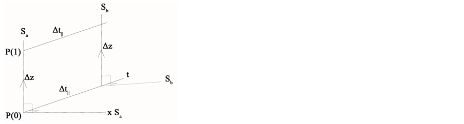
Figure 3. Parallel spatial axes. In case two different subspaces Sa and Sb have two common points P(0) and P(1), the points are part of parallel spatial axes.
3.2. Regularity in the Distances of Multiple Space
Let there be two unequal subspaces Sa and Sb both belonging to dissimilar points P(1) and P(2) meaning that both subspaces have axes pairs intersecting both points. Let there be a lot of such pairs of points and corresponding subspaces. Take of this collection two points with the same direct distance apart from the sign measured in both subspaces, a situation as illustrated in Figure 4. If x, y is the direct distance between P(1) and P(2) in subspace Sa, there is a subspace Sb in

Figure 4. Presence of a multitude of subspaces in an unit-cube. Subspaces Sa and Sb with parallel z-axis are connected via the points P(1) and P(2). Beside subspace Sb, point P(3) contains subspace . Even if
  has the same triplet of directions it cannot coincide with Sa. Consequently, within the unit-cube are several equal, non-coinciding subspaces. Next to P(1), the unit-cube includes at least x − 1 extra points.
which the same distance will be x, −y. This implies that both x-axes of Sa and Sb are perpendicular to two parallel z-axes through space-point P(1), a property that also holds for the two y axes through point P(2).
Other points on the axes between P(1) and P(2) do not share common subspaces with point P(1). Let there be a regularity in the presence of point pairs with common couple of subspaces, being a regularity on the spatial distances:
According to the second regularity of multiple space two different subspaces with parallel axes contain pairs of points on fixed direct distances measured along the perpendicular axes, independently of the perpendicular axes and the subspaces in question.
When the second regularity is true, it can be shown that the multiple space contains a huge number of both unequal subspaces and non-coincident subspaces with parallel directions. Namely, take at t (>0) the series of x points on the x-axis of Sb. At t = 0 each point is part of subspace  predominantly unequal to Sa. This series of subspaces at t = 0 forms a set of mutual unequal subspaces
 .
.
Within the spatial unit-cube Δx3 at point P(1), each subspace  is part of a space-point P´, component of a set of points {P’} (see Figure 4). This means that the points along the x-axis of Sb cause x non-coinciding points in the unit-cube. With npoint different axes of P(1), the unit-cube contains 1 + (x − 1)npoint distinguished points, not taking into account possible double counting.
When the unit-distance is universal valid in multiple space as will be shown below, the total number of points in the unit-cube is equal to the number of subspaces nsubspaces of the multiple space. Due to the (x − 1)npoint distinguished points within the unit-cube is nsubspaces? npoint. This makes that at the location of the unit-cube is present a tangle of not coincident subspaces.
3.3. Uniformity Unit-Distance across Multiple Space
For entities in a continuous space a universal measure of the distance is not self-evident, see Čapek for elucidation of the problem of the theme of Gulliver [8] . Each subspace of the multiple space has the unit-distance as distance measure, the question is whether the whole multiple space has the same measure for the distance. For this there need to be a matching between the subspaces. The first regularity provides for it.
Two subspaces of a space-point both have the same unit-distance when the axes are parallel (see Figure 3). This also applies to the subspaces of the npivot parallel axes of the space-point. Each axis, orthogonal to the npivot parallel axes, also has the same unit-distance because they belong to the same subspace. These orthogonal axes in turn have parallel axes for which the same unit-distance is applicable. Repeating the procedure makes all subspaces belonging to a point will have the same unit-distance.
A subspace is intersected by numerous points whose associated subspaces also have the same unit-distance. Because all the subspaces of multiple space somewhere are interconnected by points, the unit-distance is uniform across multiple space.
Note: With an uniform unit-distance, the theme of Gulliver is just half solved. It is also necessary that the size of physical phenomena is uniquely determined by the distances of the subspaces.
3.4. The Shortest Distance
The nsubspaces points within the unit-cube indicate a smaller mutual distance than the unit-distance. In the multiple space, the distance between two points is defined as the number of edges along the axes of the common subspace. This definition of distance cannot be used to determine the smallest distance within the unit-cube, the apparently nearest points don’t have direct connections. Indirectly there is a connection via a path over several subspaces and points whereby path-distance >> unit-distance.
In multiple space a distinction is made between the location and the position of a point. The location of a point is given by the coordinates of one of its vertices within a subspace, unique for a particular subspace. The position is determined by the fictive coordinates within a particular unit-cube, expressed in fractions of the unit-distance. To determine the position of an arbitrary point Pa within an unit-cube, take subspace Su of the unit-cube part of point Pu, and the subspace Sa of the arbitrary point on the same instant. The subspaces Su and Sa are part of a common point Pc somewhere in space. The position of Pa, a rational number, is mathematically determined by the difference of the direct distances between Pa and Pc in subspace Sa and Pu and Pc in subspace Su.
Call the virtual distance of two points within a unit-cube the difference of two positions. By taking nsubspaces points equally spread over the unit-cube, the smallest virtual distance expressed in unit-distances is of the size
 (2)
(2)
Note: A workable distance must arise out of the mutual influence of two phenomena. Interaction in multiple space probably is determined by encountering fields with the same axis direction, meaning that the meeting takes place in the same subspace. This makes that the interaction is determined by the direct distance between the entities and not by the virtual one.
4. Trigonometry and Metric from the Regularities
According to the second regularity of the multiple space, a couple of subspaces of a space point with parallel axes share a second space-point at direct distance x,y measured along the axes perpendicular to the parallel axis. The two subspaces are therefore coupled in the time and distance by the two points.
4.1. The Unit-Angle
The Consider those coupled subspaces with a minimal value of y/x and with one point on a fixed position. Since the fixed point contains npivot parallel axes, there are just as many coupled subspaces with minimal y/x. The unfixed points form an unbroken remote connection, a regular polygon if projected onto the Euclidean plane (see Figure 5). The ratio y/x can be associated with an angle which

Figure 5. Smallest angle. Projected onto R3, the axes of subspaces Sa and Sb make a so-called unit-angle when they are part of two points P(1) and P(2) having the smallest y/x ratio. The subspaces Sa and Sb have parallel z-axes at different instants in which are perpendicular the two spatial directions x and y determining the discrete-angle.
makes it possible to determine the relation between the direct distance x, y of two coupled subspaces. The arctangent of the smallest ratio of y/x is called the unit-angle αpivot expressed in radians
 (3)
(3)
A larger angle is the sum of several unit-angles. The sum of unit-angles at a point going from one space direction to the other is referred to as the discrete- angle between two directions.
The discrete-angle enables to determine the trigonometric functions of multiple space, as shown in appendix A. The variables are provided with an inaccuracy denoted by  due to the integers used
 (4)
(4)
 (5)
(5)
In which the distances a and b are the adjacent sides of a rectangular triangle, and c is the hypotenuse.
4.2. Metric Multiple Space
With the help of the discrete-angle, the direct distance in the one subspace can be expressed in direct distances of the other subspace. The discrete-angle as the coupler of subspaces together with the orthogonality of the axes enables to describe the required rectangular triangles. With these features as ingredients, the metric in accordance with the Pythagorean Theorem can be determined using the method of John Wallis’ the proof of similar triangles’ [9] . For applying these methods on the multiple space see appendix B. The variables of the Pythagorean Theorem have a small inaccuracy of the size of the unit-distance:

4.3. Geometry Regular Multiple Space versus Euclidean Geometry
Euclidean geometry is based on the empirical concepts of points, lines and planes [10] , concepts which also can be used in multiple space. In multiple space
these concepts arise from the more basic entities of vertices, edges and space structure. The geometry resulting from the concept of point and line in multiple space has features which, on a very small scale, differ from the geometry as interpreted from daily experience.
The concept of a point in multiple space and the Euclidean geometry correspond only with regard the position in space. In the Euclidean geometry, a point is continuously present during the time being the place where intersecting spatial lines meet. Random different points always have a mutual distance meaning a point has always a neighbour to be connected.
In multiple space, a point consists of a time series of connected vertices being present stepwise over time. Within the spatial unit-cube Δx3, all the nsubspaces space-points are separated with no direct connection by an edge, which means there are no connected adjacent space-points. Points are only spatially connected within a subspace over distances larger than the unit-distance Δx, meaning that random different space-points only are seldom interconnected.
In Euclidean geometry, a spatial line is a chain of points. Unless parallel, two spatial lines in a plane always intersect in a point.
Within the multiple space, a spatial line is a chain of adjacent vertices along an axis in one of the subspaces. The line is straight by definition. Different spatial line seldom intersect in a space-point, only in case the lines belong to the subspaces of the space-point. Rarely, any two space-points are part of a spatial line, namely in the exceptional case the line is an axis of a subspace. Also in case of two unit-cubes, only on a relatively short distance there is a common subspace with an axis to determine the mutual distance of the unit-cubes.
In multiple space, a curved line is a set of successive pairs of points, each pair on the axis of a common subspace. A curved line is made up of a plurality of such pairs of points. At each point there is a jump in the time of one subspace to the other. The curved line is not smooth, the line is straight on the axes of the subspaces and at each connective point there is a leap in space direction.
Depending on the definition, the concept of a plane in the multiple space differs totally from that in Euclidean space. When as an obvious possibility the plane is defined as a set of vertices determined by two orthogonal axes, the plane is present only in one subspace. By that definition, only planes in the same subspace may have an intersecting line. Arbitrary planes are present in different subspaces and thereby don’t have a line of intersecting, which is an impossibility in Euclidean geometry for non-parallel planes.
With respect to volumes, the difference with the continuous space is even more striking. In continuous space, two partially overlapping volumes always have a common volume. This is not the case in multiple space when a volume is defined as a collection of vertices within a cube of a subspace. Generally, two volumes belonging to different subspaces at about the same position have no common vertices, simply because not coincident subspaces have nothing in common. Rarely different subspaces will have common points, in which case the vertices of the subspaces are connected in the time.
The way in which the volume should be used depends on the manner objects such as fields are disposed in the multiple space.
5. Concluding Remarks
A discrete alternative for the continuous space is offered in form of a merging of a huge number of hypercubic lattices. The combined lattices provide a solution for most of the problems with the discrete space as mentioned in the introduction. The features of the multiple space are promising, the lattices give the dimensionality and the orthogonality of the axes, and the axis of merging can be interpreted as the time axis. With an appropriate choice of the regularities in the structure of multiple space, the metrical and goniometric relations match nearly perfectly those of Euclidean space.
Due to the chaos in subspaces, the multiple space is hard to fathom even with some organization by the regularities. The many unequal subspaces with three parallel axes cause that the geometry does not correspond to the perception of real space, as described in the previous chapter. This apparent discrepancy can be traced back to the ignorance how phenomena should be incorporated into multiple space.
5.1. Fields in Multiple Space
There are several possibilities to add a field to the multiple space. One possibility directly related to the conventional method is to use the multiple space as a discrete background space in which the quantities determining the field are added to the vertices of the lattice. The different lattices of the multiple space cover all possible spatial directions relative to the other lattices. By an appropriate choice of regularities, the connections between the lattices are invariable in every direction making the directions are evenly distributed. This kind of regular multiple space can act as a discrete reference space, in which each rotation across a discrete angle shows the same the same background space.
A field may also be related to the space by making use of the division of the multiple space into subspaces, making it very likely that quantities describing fields are present only in subspaces with an axis in the direction of the action of the field. Then the field is present in only npivot of the npoint subspaces in case the subspaces containing the field are coupled to a specific space-point. Another consequence of this obvious assumption is that interaction can only occur when two fields are present in the same subspaces. For the same reason, fields with different directions will not perform interaction. This also implies that, without mutual influencing, different fields may be present at about the same position in spacetime, as in the vicinity of the core of an electron. The assumption also indicates that a particle with a radially field will be present in ndirections subspaces with different triplet of directions, whereby: ndirections < nsubspaces. The advantage of the presence of a field to a limited number of subspaces is that the various characteristic of multiple space, such as npivot and ndirections, can be included in the field description, potentially giving a physical meaning to these characteristics.
5.2. The Possibility of Speed and Relativistic Effects in Multiple Space
The multiple space with some possible regularities cannot include moving phenomena or relativistic effects, since regularities affect the entire space. Namely, in the fixed frame of multiple space, speed and its effect should be a localized phenomenon having different properties with respect to other parts of the space. What remains is the possibility that deviations of the space structure will cause different behaviour of spatial enclaves.
It can be shown that there are possible deviations of the lattice structure in the upper and bottom plane of a spatial cube L3 which will have an impact on the axes of the embedded cube. Within the cube the time axis and one of the spatial axes are not parallel to those of the surrounding space. Following the development in the time, the cube moves relative to the surroundings with a speed v = 1/L forming an inclined corridor in the time. To put it more vividly: the deviations seem to annihilate the surrounding space on the upper plane in order to change it into a moving cube, and subsequently to restore the surroundings at the lower plane at the expense of the moving cube.
A side effect of the moving cube is that the enclosed space is deformed such that the spacetime in the cube has relativistic properties with respect to the surrounding space. The deformation of space is needed to ensure that the spacetime density of the vertices is the same both in and outside the time-corridor of the cube. At the four boundary surfaces of the time-corridor, each vertex has to have eight edges in all spatial directions as connections with other vertices both in and outside the cube. Within the time-corridor of the cube, the space has the shape of a lattice.
Cite this paper
de Groot, C.T. (2017) A Euclidean-Like Discrete Spacetime from the Unification of a Multitude of Hypercubic Lattices. Journal of Modern Physics, 8, 1175-1189. https://doi.org/10.4236/jmp.2017.88078
References
- 1. Smolin, L. (2005) Scientific American Special Edition, 15, 56-66.
- 2. Rothe, H.J. (1992) Lattice Gauge Theories: An Introduction. World Scientific, Singapore, 32-36.
- 3. Forrest, P. (1995) Synthese, 103, 329-330.
https://doi.org/10.1007/BF01089732 - 4. Grünbaum, A. (1974) Philosophical Problems of Space and Time. Reidel, Dordrecht, 209, 336.
- 5. Van Bendegem, J.P. (1987) Philosophy of Science, 54, 295-302.
https://doi.org/10.1086/289379 - 6. Meschini D. (2006) Geometry, pregeometry and beyond. Foundations of Physics, 36, 1193-1216.
https://doi.org/10.1007/s10701-006-9058-8 - 7. Rosen, K. (2000) Handbook of Discrete and Combinatorial Mathematics. CRC Press, Boca Raton, 495-595.
- 8. Capek, M. (1961) The Philosophical Impact of Contemporary Physics. Van Nostrand, Princeton, New Jersey, 21-22.
- 9. Dunham, W. (1994) The Mathematical Universe. Wiley, New York, 93-95.
- 10. Robinson, G. (1963) The Foundations of Geometry. University of Toronto Press, Toronto, 9-13.
Appendix A. Trigonometric Functions in Multiple Space
Take two subspaces S1 and S2 of point PA with a parallel axis (z-axis). The axes x1 and x2 of both subspaces orthogonal to z form an angle. See Figure 6 for orientation. In S1 the points PA, PB1, PC1 are part of a rectangular triangle with a and b the direct distances. In S2, c is the direct distance between points PA, PC2. Because S1 and S2 are different subspaces, points PC1and PC2are generally not equal, except in the case of a Pythagorean triple.
Let the distances a, b and c be such that the points PC2 and PC1 are within the same unit-cube. Take the rectangular triangle PA, PB1, PC2 of the combined subspaces. With an average inaccuracy of , the distance in the one subspace expressed in the other is


From which the trigonometric functions (4) and (5) follow.
Remark:
The trigonometric functions (4), (5) apply to the angles between axes converging in one point. For not converging axes, the spatial angle can be defined as the angle between any two spatial axes through various points within an unit- cube.
Let two subspaces S1 and S2 be part of different points PA1 and PA2 present in one unit-cube. Both subspaces are also part of points PC1 and PC2 in another unit-cube. In S1, the position of point PC1 relatively to PA1 is described by a, b. In S2, the direct distance between PA2 and PC2 is c. With points PA1 and PA2 in the one unit-cube and PC1 and PC2 in the other, there are two inaccuracies in the positioning which can be expressed by the same .
.

Figure 6. Trigonometric functions. Point PA contains two subspaces S1 and S2 with parallel z-axes. The x- and y-axes of subspaces S1 and S2 are perpendicular to the two parallel z-axes. Therefore, lines a, b, c are located on a flat plane when projected on S1. The x1 and x2-axes form an angle. The two points PC2 in S2 and PC1 in S1 are present in one unit-cube. From the sketched situation can be obtained the trigonometric functions with a numerical inaccuracy of the size of the unit-distance.
Appendix B. Metric Multiple Space
Take the subspaces S1 and S2 of point PA with parallel z-axes. Perpendicular to the z-axis of S2 are two orthogonal axes with discrete-angles α and β relative to those of S1. The points PA, PB1 and PC1 on the orthogonal axes of S1 form a rectangular triangle. The distances along the various axes are so that point PB2 of S2 is in the same unit-cube as PB1, making c the hypotenuse of the adjacent sides a and b of the triangle PA, PB2, PC1. Using (4) and (5), these distances are related as  and
and  (see Figure 7(a)).

Figure 7. Derivation of the pythagorean theorem. Subspaces S1 and S2 of point PA have parallel z-axes and thereby a discrete-angle divided into the angle α with the y-axis and angle β with the x-axis. In S1 the distances a and b are sharply defined, in S2 the distance c is exact. The non-coincident points PB1 and PB2 are situated in an unit-cube. Consequently, a and b can be expressed in c with an inaccuracy of . The same applies to the relation between a2 and a as well as b2 and b.
The axis of d2also is perpendicular to the z-axis of S2. Let d2have such a length that points PC1 and PC2 are situated within an unit-cube. This implies that the distances a and b are the adjacent sides of two rectangular triangles with common side d2 making  and
and  (see Figure 7(b)). By eliminating α and β and using
 , the Pythagorean Theorem of multiple space becomes:


Submit or recommend next manuscript to SCIRP and we will provide best service for you:
Accepting pre-submission inquiries through Email, Facebook, LinkedIn, Twitter, etc.
A wide selection of journals (inclusive of 9 subjects, more than 200 journals)
Providing 24-hour high-quality service
User-friendly online submission system
Fair and swift peer-review system
Efficient typesetting and proofreading procedure
Display of the result of downloads and visits, as well as the number of cited articles
Maximum dissemination of your research work
Submit your manuscript at: http://papersubmission.scirp.org/
Or contact jmp@scirp.org