Journal of Modern Physics
Vol.5 No.7(2014), Article ID:45543,13 pages
DOI:10.4236/jmp.2014.57066
Diagrammatic Iteration Approach to Electron Correlation Effects
J. D. Fan1,2, Y. M. Malozovsky2,3
1Chongqing Center for Superconductive Science & Technology, Chongqing Academy of Science and Technology, Chongqing, China
2JD Duz Institute for Superconductivity, Baton Rouge, USA
3Department of Physics, Southern University and A&M College, Baton Rouge, USA
Email: 1097420465@qq.com, omaloz@cox.net
Copyright © 2014 by authors and Scientific Research Publishing Inc.
This work is licensed under the Creative Commons Attribution International License (CC BY).
http://creativecommons.org/licenses/by/4.0/


Received 16 January 2014; revised 18 February 2014; accepted 12 March 2014
ABSTRACT
Electron correlation is a measure of the errors that are inherent in the Hartree-Fock theory or orbital models. When the electron density is high, correlation is weak and the traditional electronic theory works well. However, at a low density of electrons correlation effects become strong and the traditional theory fails to describe the electron system correctly. Therefore, the electron correlation plays a radical role in such materials as high-temperature superconductors and heavy fermions, etc. To date, there is no agreement on how to deal with higher-order terms (correlation energy) in the series of electron’s ground state energy although a method that is termed diagrammatic iteration approach (DIA) was developed more than one decade ago by the authors of this article. That is why no consensus on the origin and mechanism of superconductivity has been engaged in superconductivity community. From the viewpoint of methodology, the DIA is indeed an approach to higher-order terms from the lower-order ones, i.e. it is a new method to show how to go beyond the random phase approximation (RPA) step by step by iteration. Here, we are logically presenting it to the community of modern physics with more analyses and hope to attract more attention to it and promote its applications.
Keywords:Electron Correlation Effect, Diagrammatic Iteration Approach, Superconductivity, Condensed Matter Physics

1. Introduction
Nowadays, looking around theoretical literatures of condensed matter physics, it is obvious that methodology of dealing with an electron system remains to be based on the Hartree-Fock (HF) theory plus a variety of approximations that are used to estimate the correction of electron correlation effects to the total energy of the electron system and other relevant properties caused by the correlation. In the case of a high-density electron system like a metal or alloy the conventional electronic theories work well, but it fails to provide correct information to interpret and understand phenomena observed in experiments with a low-density electron system, such as a hightemperature superconductor (HTS). The long-term arguments existing in the community of superconductivity on the mechanism of a high transition temperature since 1986 after the discovery of the first superconductor of the cuprate type are attributed to the lack of sufficient attention to the need of a developed many-particle theory that is capable of well treating the electron correlation effects. It seems that the great success of conventional electronic theories in terms of the mean field approach (MFA) in metals, semiconductors and many other fields of condensed matter physics leads one to attempt to polish the existing conventional theories for explaining and understanding the “anomalies” observed with cuprate superconductors, where the word of anomaly is relative to the observations from conventional superconductors. The anomalies are, as a matter of fact, the natural outcomes of a cuprate superconductor at specified conditions. They should be derived from an elaborate and sophisticated theory accounting for the electron correlation effects. Although we had worked out a theory in terms of the diagrammatic interaction approach (DIA) more than one decade ago to deal with superconductivity regardless of highor low-transition temperature [1] , yet a little attention was paid to it to date. Now, we believe that the DIA we developed is a powerful theoretical weapon in condensed matter physics, and not only applicable to superconductivity, but also very useful in the areas where correlation is appreciable.
2. A Brief Review
2.1. Second Quantization for Particles
For the routine discussions and derivations of second quantization for a particle system we use the results from Gerald D. Mahan [2] .
The full electron gas Hamiltonian is often too complicated to use for the more elaborate many-body theory. Quite often this is approximated by a model Hamiltonian which has a simple form. Usually, these model Hamiltonians look very simple but it still impossible to solve them exactly. Often it is even difficult to solve them approximately!
The homogeneous electron gas is a model that is frequently used to learn about electron correlation effects. The homogeneous model is also called Jellium model. We can think of taking the positive charge of the ions and spreading it uniformly about the unit cell of the crystal. Of course, the homogeneous electron gas then has no crystalline structure. It has the Hamiltonian
 (1)
(1)
where the first term is kinetic energy and the second represents pair interactions between two particles with spins of σ and σ'. Moreover, vq in Equation (1) is the representative of the Coulomb interaction in k-space and usually thought of as the Fourier transformation, equal to 4πe2/q2, of the Coulomb interaction V(r) = e2/r. It seems that there is nothing wrong here, but the problem is just from here as shown elsewhere [3] , in which we have proved that there is a sign reversal of the Coulomb interaction in k-space due to correlation effects. Therefore, if we wish to take into account many-body correlation effects, vq here is no longer that simple.
Since Equation (1) stays insolvable, we has to manage to simplify it gain. For example, if we adopt the socalled Cooper’s pairing condition of k + k' = 0 and σ + σ' = 0 as said in the BCS (Bardeen-Cooper-Schrieffer) theory [4] , the BCS Hamiltonian is obtained as below [5] .
 (2)
(2)
However, even if the Hamiltonian has been further simplified with the Cooper’s pairing condition, it remains unresolvable because of the complicated and unknown interaction V(k, k'). The simplification of BCS [4] is to assume V(k, k') = −|V|, a constant, and get a solution to Equation (2), leading to a rather good result of the isotope effect exponent α = 0.5 due to the use of the Debye frequency ωD to be the cutoff frequency. This outcome of α = 0.5 fits to the experimental data observed then from some conventional superconductors. The assumption and simplification of V(k, k') to be the negative constant forces BCS to accept another rather strange concept— attractive interaction between two electrons due to the mediation of phonons! If V(k, k') is positive, there would be no solution at all to the BCS Hamiltonian. This paradoxical concept has confused us for more than half a century and was eventually proved to be improper [3] . Yes, V(k, k') must be negative, but it is due to the correlation effects of electrons, instead of phonons. Moreover, V(k, k') is the pair interaction between two quasielectrons in momentum space. The sign reversal of Coulomb’s interaction in momentum space is just the consequence of many-electron correlation effects. In contrast, if the negative interaction stems from phonon mediation, which is possible when Coulomb screening is strong enough in the case of a dense electron system like a metal, the transited state would be insulating, instead of superconducting [6] -[10] .
2.2. Interelectronic Coupling
There are two electronic properties that are important: the self-energy of an electron of momentum p and the total energy of the N-electron system.
First of all, the inter-electronic coupling constant is defined as
 (3)
(3)
where e—electron charge, —Fermi velocity,
 —Fermi momentum with the
convention of assuming
—Fermi momentum with the
convention of assuming
 to be a unit, and
 —the effective Bohr radius
with ε being the dielectric constant. It is known that
—the effective Bohr radius
with ε being the dielectric constant. It is known that
 (3D)(4.a)
and
 (2D), (4.b)
where n and ns are the density of electrons in 3D and 2D, respectively.
It can be seen that the higher the density of electrons, the smaller the coupling
constant. The condition of
 corresponds to weak coupling, as it is in a conventional metal, while the fact that
α~1 or ? 1 represents an intermediate or strong coupling case as observed, for example,
in cuprate superconductors. The conventional electronic theory based on RPA or local
density approximation is, strictly speaking, valid for the case of weak coupling
only. For many metals RPA is a good approximation and conventional electronic theory
works very well because the density of electrons in the metals is generally large
enough to ensure a small coupling constant α. The conventional superconductors can
also be well described by the BCS theory [4] except for the concept of electron-phonon
interaction leading to attraction between two electrons. However, the category of
cuprate oxides superconductors are formed due to doping, the density of carriers
(electrons or holes) is always so low that the interelectronic coupling constant
is quite large.
corresponds to weak coupling, as it is in a conventional metal, while the fact that
α~1 or ? 1 represents an intermediate or strong coupling case as observed, for example,
in cuprate superconductors. The conventional electronic theory based on RPA or local
density approximation is, strictly speaking, valid for the case of weak coupling
only. For many metals RPA is a good approximation and conventional electronic theory
works very well because the density of electrons in the metals is generally large
enough to ensure a small coupling constant α. The conventional superconductors can
also be well described by the BCS theory [4] except for the concept of electron-phonon
interaction leading to attraction between two electrons. However, the category of
cuprate oxides superconductors are formed due to doping, the density of carriers
(electrons or holes) is always so low that the interelectronic coupling constant
is quite large.
2.3. Characteristic Length rs
Another important dimensionless parameter rs, characteristic length of the system of interest, is adopted to be a criterion of the electron density, and defined as below
 ,(3D)
(5.a)
,(3D)
(5.a)
 (2D)
(5.b)
(2D)
(5.b)
where
 is the radius of the sphere in Bohr radius units, in which an electron charge is
enclosed. It can be seen that the higher the density n or ns, the smaller
the parameter rs. In terms of this definition, kinetic energy Ek
is calculated to be
is the radius of the sphere in Bohr radius units, in which an electron charge is
enclosed. It can be seen that the higher the density n or ns, the smaller
the parameter rs. In terms of this definition, kinetic energy Ek
is calculated to be
 (3D) or
 (2D) [2] , whereas the interaction part in the ground state energy is divided into
two parts: exchange and correlation. The exchange part has been exactly calculated
for Coulomb interaction
(2D) [2] , whereas the interaction part in the ground state energy is divided into
two parts: exchange and correlation. The exchange part has been exactly calculated
for Coulomb interaction
 in 3D case and
 (2D). The second part, however, was estimated [11] -[15] in RPA or in terms of the
generalized RPA including the well-known Hubbard correction (see the so called Hubbard
local field factor) which explicitly accounts for the exchange and short-range correlations,
i.e., only the single scattering between electrons is taken into account among the
possible scattering patterns between electrons. The efforts were made to calculate
each contribution. The result for the ground state energy per electron Eg
is given by [2] .
(2D). The second part, however, was estimated [11] -[15] in RPA or in terms of the
generalized RPA including the well-known Hubbard correction (see the so called Hubbard
local field factor) which explicitly accounts for the exchange and short-range correlations,
i.e., only the single scattering between electrons is taken into account among the
possible scattering patterns between electrons. The efforts were made to calculate
each contribution. The result for the ground state energy per electron Eg
is given by [2] .
 (6.a)
(6.a)
for 3D and
 (6.b)
(6.b)
for 2D, where the first term is kinetic energy, the second is the exchange energy, and all of the rest terms together construct the correlation energy Ec. In Equation (6.b) εr is the so-called ring energy, which is usually evaluated approximately in consideration of the ring-diagrams and the second-order exchange diagrams. Many authors have also obtained the results shown in Equations (6.a) and (6.b) [3] [11] -[16] .
It is seen that when the density of electrons is high (rs = 1), kinetic energy prevails the potential energy (exchange and correlation energies) and the latter is hence negligible. Thus, the free-particle model works well and the corresponding results from the free-particle model are accurate. The conventional perturbation theory was developed based on the free-electron model. It is obvious that the free-electron model is good for such a high electron density as it is in a conventional metal, but not accurate for a low density of electrons in which rs is close to or greater than 1 and the coupling constant α is also greater than 1. It is easy to see that when rs > 2, |Ex| > Ek. Therefore, as the density of electrons keeps decreasing, Ec is no longer negligible, nor is the free particle model valid.
2.4. Correlation Effects
The different types of the elastic or inelastic, magnetic (spin-dependent) or non-magnetic processes of scattering may cause electrons to become localized or nearly localized. In particular, if the material under investigation has a low density of electrons and/or a high density of defects (or impurities), inter-electron coupling constant α is close to or greater than 1. Meanwhile, the parameter characterizing the scattering of electrons kE l is also close to 1, where kF is the Fermi momentum and l = vF τ is the mean free path.
Therefore, strictly speaking, the conventional treatment of electrons in bulk electronic materials does not apply to a dilute electron gas because the methods, based on the use of the lowest order of perturbations, i.e., the RPA in interaction and the Born approximation in scattering, are no longer valid for this case where correlation effects play a major role since these methods treat electrons as if they were free. In other words, the so-called vertex correction—higher-order correction in the self-energy part or two-electron interaction kernel, while using diagrams, must be taken into account. The incorporation of correlation in the interaction (scattering) allows us to expand the existing methods and to develop a new method in electronic theory. The question is how we can go beyond the RPA approximation with the diagrammatic method.
It is also well known [16] that correlation effects in a low dimension are enhanced due to the reduction of freedom of motion. Therefore, RPA is inadequate in a low dimension even though the coupling constant may be still so small that the problem seems to pertain to the regime of week coupling, where the conventional electronic theory works well.
3. Diagrammatic Iteration Approach
3.1. Methodology
In general, there are two methods to deal with an electronic system: Hamiltonian and quantum field theory. Conventionally, we in general seek a proper Hamiltonian for a system of particles and then find out its approximate solution. The BCS theory is a good example of the attempt of this kind for conventional superconductors. The Hubbard model with a large positive constant U which has been believed to be the Hamiltonian appropriate for HTS looks simple enough, but to date a solution to it was obtained only in one dimension. Therefore, even if the assumption of a constant interaction potential is valid in some special cases, we are still in the difficulty of obtaining its solution. The major issue here is how much we can do with a Hamiltonian and how much information we are able to extract from it.
Nevertheless, the quantum field theory appears to be better in dealing with a many-particle system in the case of strong coupling. By means of the diagrammatic method, if we manage to construct an equivalent diagram for the interaction potential energy and then converts it to an integral equation, we can get the transition condition by the pole condition of the equation, which corresponds to a phase transition.
The difficulty we meet in trying to go beyond RPA, however, rests in the lack of an acceptable approach to take into account higher-order corrections to the self-energy of a single electron due to correlations. The partial summation that has been used in this approach often give rise to diverse and sometimes controversial outcomes and conclusions because some of the higher-order terms may be canceled out and a partial summation may happen to pick up only the terms that lead to divergence. A survey of literature on superconductivity theory during the past two decades clearly shows a severe shortage of the works based on quantum field theory. Its importance in condensed matter physics is unquestionable since it is the only way to approach the detailed information of interactions of a many-particle system.
3.2. Introduction to Diagrammatic Iteration Approach
In weak coupling, it is well known that the Hamiltonian method is in good agreement with the diagrammatic approach. For example, in the study of superconductivity the BCS theory [4] and the Eliashberg theories [17] give rise to consistent results. In strong coupling, however, the Eliashberg theory fails as the BCS theory does. Therefore, in order to obtain a result beyond RPA a technique to be used to go beyond RPA must be developed. The diagrammatic iteration approach was hence born in our previous work [1] based on quantum field theory in terms of the well-known Ward’s identity. For completeness of this article we present the essential part of DIA here without much repeating the part pertaining to superconductivity. As a generic method, DIA can be employed in any field where correlation effects play an important role.
Now, let us brief the methodology of DIA. The well-known Migdal’s expression [17] -[19] for the single-particle self-energy incorporating the vertex part can be written as
 (7)
(7)
where p and k are the four-dimensional vectors, G(k) and D(k) are the dressed electron
and boson Green’s functions, respectively. The boson Green’s function satisfies
the so-called Dyson equation
 with D0(k) being the zeroth-order boson Green’s function, and
 being the irreducible polarizability that has the standard form as given below [18]
[19] . For example, in the case of the Coulomb interaction
being the irreducible polarizability that has the standard form as given below [18]
[19] . For example, in the case of the Coulomb interaction

where V(k) is the matrix element of the bare Coulomb interaction. In the case of the electron-phonon interaction

where
 and
and
 are the unrenormalized (original) matrix element of the electron-phonon interaction
and the phonon characteristic frequency, respectively. The irreducible polarizability
is given by
are the unrenormalized (original) matrix element of the electron-phonon interaction
and the phonon characteristic frequency, respectively. The irreducible polarizability
is given by
 (8)
(8)
where Γ(p, k) is the three-point vertex function and, in the ladder approximation, is defined as [17] -[21] .
 (9)
(9)
where K(p, p') denotes the kernel of the integral equation for the vertex function
and describes the many-particle correlations. The interaction kernel K(p, p') in
Equation (9) satisfies Ward’s identity [18] [19] and can be therefore written as
a functional derivative of the self-energy with respect to the electron Green’s
function,
 which depends, in general, on the spin indices. The nonlinear system of Equations
(7)-(9) gives a complete consideration of the problem.
which depends, in general, on the spin indices. The nonlinear system of Equations
(7)-(9) gives a complete consideration of the problem.
The DIA’s core is iteration. Namely, starting from the known information—the single-particle self-energy in RPA, wherein Γ is taken to be 1, we obtain the two-particle interaction kernel K in terms of Ward’s identity,

where G is Green’s function of electron and p four-dimensional momentum and σ spin. Then, with the newly obtained K and the RPA’s Γ = 1 we can calculate the vertex part Γ according to Equation (9), in the first step beyond RPA. The vertex part obtained here can be substituted into Equation (7) for Γ to re-calculate the selfenergy and then the interaction kernel K based on Ward’s identity at the first step beyond RPA. By now, the first loop of the iteration has been completed and all of the quantities of Σ, K and Γ in the first step beyond RPA have been calculated. The second loop is that in terms of the self-energy Σ and the vertex Γ obtained in the first step beyond RPA we are able to recalculate K and Γ in the second step beyond RPA, and then Σ again. Thus, the second loop is completed. Of course, from Equation (8) irreducible polarizability can also be calculated in each step in terms of the corresponding vertex part Γ. By doing so step by step we can sequentially receive all the possible information in principle to any step beyond RPA. However, mathematical complexity makes it unrealistic to do so analytically to higher orders. Of more difficulty is that we are unable to get the summation of the complicated kennels of all the orders even if we could get several analytic expressions. Thus, no success has been made analytically. Instead, a diagrammatic technique is recommended.
Based on Feynman’s diagrammatic symbols used in quantum filed theory: a solid line
with an arrow directed on one side represents Green’s function of an electron and
a dashed one stands for Green’s function of a boson, we may construct the diagram
of the spin-dependent single particle self-energy
 as shown in Figure 1, where the left diagram corresponds
to Equation (7) and the right one is its approximation in RPA in which Γ(p,k) is
taken to be 1.
as shown in Figure 1, where the left diagram corresponds
to Equation (7) and the right one is its approximation in RPA in which Γ(p,k) is
taken to be 1.
In Figure 1, the black corner is termed the vertex correction, which is negligible in the weak coupling of electron-phonon interaction as proven by Migdal [19] . The dashed line representing a boson field is understood as a dressed line under the RPA assumption. The well-known Eliashberg theory is based on this diagram in Figure 1(b).
However, when coupling is strong, from the viewpoint of the diagrammatic method, the high-order corrections are no longer negligible and the problem now becomes how to find out diagrammatic structure of the vertex function. In principle, there are infinite number of Feynman diagrams that represent all of the possible interaction patterns. Of more importance is now to have a rule or regulation of constructing them. An intuitive way is to follow the order of the boson line. A preliminary evaluation shows that the convoluted relationship among the self-energy Σ interaction kernel K and the vertex function Γ leads to a variety of developments of the diagrams as shown below, and the weight of each of the diagrams, even if they are in the same order, is different and that the contribution from a diagram in a higher order may be larger than that from a low-order diagram. A variety of partial summations may lead to completely different or conflict results. Therefore, only a complete summation all over the possible diagrams is reliable and acceptable. To this end we have developed a method to reach this goal going out of RPA step by step. This is the so-called diagrammatic iteration approach briefly described as below.
In order to do so he first thing needed is to find the diagrammatic functional derivative
operation. Clearly, from the mathematical definition of a derivative the functional
derivative with respect to the electron Green’s function
 can be represented by a cut diagrammatically on the solid line that stands for the
electron Green’s function. If a diagram containing a solid line represents the self-energy,
the resulting new diagram after being cut and starched out should represent the
corresponding interaction kennel. This is consistent with
can be represented by a cut diagrammatically on the solid line that stands for the
electron Green’s function. If a diagram containing a solid line represents the self-energy,
the resulting new diagram after being cut and starched out should represent the
corresponding interaction kennel. This is consistent with .
.
It is worthwhile to indicate that we may have two different models in dealing with the interaction potential: a given or renormalized interaction. The first model means a simple boson propagator represented by a dashed line as shown on the right hand side of Figure 1. The second model takes into account contributions from particle-hole excitations, which are represented by a solid loop on the dashed line as shown on the top diagram of Figure 2.
 (a) (b)
Figure 1. Diagram of the spin-dependent single particle self-energy, Σs(p), (a) and its RPA representation (b).

Figure 2. Diagrammatic functional derivatives of the RPA diagram of the self-energy with respect to the electron Green’s function in the model with a renormalized interaction due to particle-hole excitations.
For the first model—a given interaction, by means of the diagrammatic functional derivative technique a cut on the electron line of the RPA self-energy diagram on Figure 1(a) obviously results in the first-order exchange interaction kernel as shown by the diagram (a) on the top of Figure 3, in terms of which we can construct the vertex part as displayed by the second diagram on the top right of Figure 4(a) and the corresponding self-energy diagram with the vertex correction represented by the right diagram of the first row on Figure 4(b). There are now three sections of the electron’s solid line to be cut on this diagram as shown on the bottom of Figure 3, producing other three sub-diagrams of the interaction kernel. Two of them are the same and shown by the middle one, denoted by (b, c), on the top of Figure 3. The rightest, denoted by (d), on the top of Figure 3 represents the third one. In terms of those three newly obtained sub-diagrams of the interaction kernel we can construct the rest three sub-diagrams of the self-energy with the corresponding vertex corrections on the bottom of Figure 4(b).
However, for the second model—a renormalized interaction, a cut of any electron
line on the RPA diagram of , including the electron-hole
excitation loop, is shown in Figure 2 by a wavy
line (a, b & c). Each of the cuts corresponds to a functional derivative
, including the electron-hole
excitation loop, is shown in Figure 2 by a wavy
line (a, b & c). Each of the cuts corresponds to a functional derivative , giving rise to a sub-diagram of the interaction
kernel. Diagrams a, b, & c coming from cutting at a, b & c in
, giving rise to a sub-diagram of the interaction
kernel. Diagrams a, b, & c coming from cutting at a, b & c in
 are shown on Figure 2. It is seen that for the
second model the situation is more complicated than the first one. However, we do
not plan to go further with it in this article and wish to focus our attention on
the first model that is relatively simpler than the second to showcase how to figure
out electron correlation effects grammatically based on DIA.
are shown on Figure 2. It is seen that for the
second model the situation is more complicated than the first one. However, we do
not plan to go further with it in this article and wish to focus our attention on
the first model that is relatively simpler than the second to showcase how to figure
out electron correlation effects grammatically based on DIA.
For a given interaction, first of all, we try to go beyond RPA analytically.
Taking into account the spin index in Equation (7), assuming D(k) = D0(k) and Γ(p, k) = 1 in it, and using the
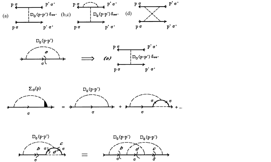
Figure 3. The graphical functional derivatives
of the diagrams for the selfenergy incorporating the first-order vertex correction
with respect to the electron Green function in the model of a given interaction
(a), ((b), (c)) and (d). Cutting any electron line in a diagram for Σs(p)
is shown by a wavy line and corresponds to the functional derivative . The cutting leads to the
following diagrams: (a) the first-order exchange interaction; ((b), (c)) the first-order
exchange interaction incorporating the vertex correction of the first-order; (d)
the diagram with crossed boson lines. The broken lines stand for D0(k),
a given interaction.
. The cutting leads to the
following diagrams: (a) the first-order exchange interaction; ((b), (c)) the first-order
exchange interaction incorporating the vertex correction of the first-order; (d)
the diagram with crossed boson lines. The broken lines stand for D0(k),
a given interaction.
 (a)
(a) (b)
(b)
Figure 4. (a) The diagram representation of the vertex part Γ(p,k) and (b) the spin-dependent single-particle self-energy Σs(p) in the model of a given interaction. The dashed lines are the same as in Figure 3.
identity
 for Ward’s relation
 , we derive the expression
for the kernel in the first step (the first order as well in this case) beyond RPA
as
, we derive the expression
for the kernel in the first step (the first order as well in this case) beyond RPA
as
 (10)
(10)
Substituting Equation (9) with the spin indices and the kernel of Equation (10) into Equation (7), we obtain the self-energy incorporating the vertex correction in the first step (order) beyond RPA. Using Ward’s identity one more time for the single-particle self-energy that incorporates the vertex correction with the kernel of Equation (10), we express the interaction kernel up to the second step (order) as
 (11)
(11)
where
 is given by Equation (10),
 (12.a)
and
 (12.b)
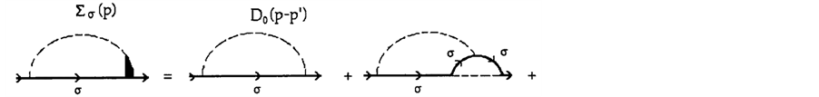
Instead of doing so further, we use diagrams to represent the above equations. The diagrams for these interactions are given in Figure 3. Also, for clarity, we redraw Figure 5, where the bisection (cutting) of any electron line is introduced to represent the procedure of the diagrammatic (graphical) functional derivative
 . It is seen from Figure 5
that the diagram (a) corresponds to the first order exchange interaction, whereas
two others, (b, c) and (d), correspond to the second order. As a matter of fact,
the diagram (b, c), K2(p, p'), corresponds to the first order exchange
interaction incorporating the vertex correction of the first order. The last diagram
(d), (
. It is seen from Figure 5
that the diagram (a) corresponds to the first order exchange interaction, whereas
two others, (b, c) and (d), correspond to the second order. As a matter of fact,
the diagram (b, c), K2(p, p'), corresponds to the first order exchange
interaction incorporating the vertex correction of the first order. The last diagram
(d), ( , in Equation (12.b)), the so-called
“crossed” diagram, is very important because it represents the interaction in the
Cooper channel for a superconductor and leads to the well-known logarithmic singularity
of the two particle vertex function [4] [18] [22] in the case of an attractive
, in Equation (12.b)), the so-called
“crossed” diagram, is very important because it represents the interaction in the
Cooper channel for a superconductor and leads to the well-known logarithmic singularity
of the two particle vertex function [4] [18] [22] in the case of an attractive
 (a)
(a)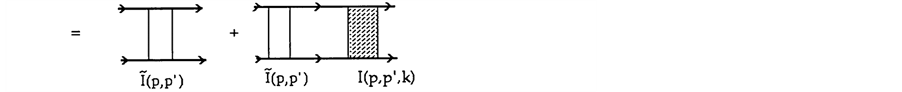 (b)
(b)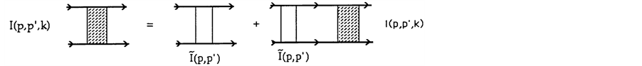 (c)
(c)
Figure 5.
The diagram representation in the model of a given interaction: (a) the interaction
kernel K(p, p') in the particle–particle channel up to the second order; (b) a series
of the ladder diagrams corresponding to K(p, p') and (c) the diagrammatic equation
for I(p, p', k), the effective two-particle vertex function. The broken lines stand
for a given interaction. The two vertical lines represent
 the irreducible interaction kernel, and the hatched area stands for I(p, p', k),
the effective two-particle vertex function.
the irreducible interaction kernel, and the hatched area stands for I(p, p', k),
the effective two-particle vertex function.
interaction D0(k) < 0. The diagrams of the vertex part & the self-energy with the interaction kernel, described by Equation (11) and Equation (12), are given in Figure 4.
As an example, we can evaluate kernels K2 (p, p') and K3 (p, p') in the case of the non-retarded interaction, i.e., when D0(k) = D0(k), where D0(k) is a given frequency-independent interaction. If we assume that the electron Green’s function is given by

where
 is the single-particle energy measured relative to the chemical potential. This
implies that we use Green's function of a perfect Fermi gas. After the frequency
summation Equation (12.a) and Equation (12.b) turn to the forms, respectively
is the single-particle energy measured relative to the chemical potential. This
implies that we use Green's function of a perfect Fermi gas. After the frequency
summation Equation (12.a) and Equation (12.b) turn to the forms, respectively
 (13.a)
and
 (13.b)
where
 is omitted. Equation (13.b) indeed has a logarithmic singularity~
 for
for

where
 is the characteristic cutoff energy of the given interaction.
3.3. An Application of DIA to a Given Interaction in an Isotropic 3D Gas
According to the above descriptions and skills introduced on Figure 3 and Figure 4, we are able to draw the diagrams of interaction kernels up to any order as shown in Figure 5 in which only those diagrams up to the second order are presented. Sorting the diagrams of interaction kernels in Figure 5 and finding out the construction rule, we are able to make a diagrammatic summation all over the possible interaction (scattering) diagrams (patterns) and hence get the diagrammatic equation of I(p, p', k), which is as well in a convoluted format like Dyson equation and represents the resulting two-particle interaction (Figure 5). Of course, in the detailed treatment more cares should be taken of and more skills are needed.
Let us replace the kernel by the effective two particle interaction,
 , equivalent to the two-particle vertex part
 in the Fermi liquid theory [18] [21]
[22] . Now, according to Equation (9), we can easily write down the vertex part with the interaction kernel replacement of I(p, p', k) as
 (14)
(14)
To evaluate , the effective two particle
interaction, we consider Equations (11) and (12) for
, the effective two particle
interaction, we consider Equations (11) and (12) for
 and its diagram representation shown in Figure 3.
To represent the interaction in the particle-particle channel, we twist all upper
lines in Figure 3 and make a series of the ladder
diagrams as shown in Figure 5(a). Further, to carry
out the ladder summation of all diagrams we can replace the first two diagrams by
the irreducible kernel
and its diagram representation shown in Figure 3.
To represent the interaction in the particle-particle channel, we twist all upper
lines in Figure 3 and make a series of the ladder
diagrams as shown in Figure 5(a). Further, to carry
out the ladder summation of all diagrams we can replace the first two diagrams by
the irreducible kernel
 as shown in Figure 5(b), where
 is the sum of all the scattering diagrams that cannot be divided by a vertical line
into two parts which are joined by two electron lines directed to one side [18]
[22] . In the lowest order
is the sum of all the scattering diagrams that cannot be divided by a vertical line
into two parts which are joined by two electron lines directed to one side [18]
[22] . In the lowest order

where
 and
and
 are given by Equations (10) and (12.a), respectively. The diagram representation
of
are given by Equations (10) and (12.a), respectively. The diagram representation
of
 is shown in Figure 5. As a result, the equation
for it can be written as [4] [18] [22]
is shown in Figure 5. As a result, the equation
for it can be written as [4] [18] [22]
 (15)
(15)
We consider the case when the given interaction is similar to the electron-phonon
interaction, i.e.
 . Now, We can evaluate
 , the irreducible kernel
of interaction, and consider
, the irreducible kernel
of interaction, and consider
 which, from Equation (12.a), can be written as
 (16)
(16)
We first consider the case of , where the characteristic boson
cutoff frequency is much less than the Fermi energy. Carrying out both the frequency
summation in Equation (16) in the region
, where the characteristic boson
cutoff frequency is much less than the Fermi energy. Carrying out both the frequency
summation in Equation (16) in the region and the integration with respect to
 , where
 is the characteristic cutoff momentum of the boson spectrum), we can approximate
Equation (16) for
is the characteristic cutoff momentum of the boson spectrum), we can approximate
Equation (16) for
 as
as

where
 is the electron-boson interaction constant. λ is related to
 , the dimensionless electron-boson
interaction constant, as
, the dimensionless electron-boson
interaction constant, as
 with
with

and the density of states per spin NF (for example, in an isotropic 3D or 2D electron spectrum
 or
or , respectively, where m*
is the effective mass and pF is the Fermi momentum).
, respectively, where m*
is the effective mass and pF is the Fermi momentum).
 given by Equation (16) is small for
 . Thus, we can estimate
 as
as
 and confine ourselves to the simple first-order vertex,
i.e.,
and confine ourselves to the simple first-order vertex,
i.e.,
 when
when . This is in agreement with
the Migdal theorem [18] [19] . It is seen that due to the fact of
. This is in agreement with
the Migdal theorem [18] [19] . It is seen that due to the fact of
 this conclusion is valid even without assuming that λ (or
 ) is small. In the case that
 is not small (i.e.,
 ), the irreducible kernel can
be approximated as
), the irreducible kernel can
be approximated as

where
 is the effective electron-boson interaction constant. This implies that the vertex
correction does affect the electron-boson interaction constant when
is the effective electron-boson interaction constant. This implies that the vertex
correction does affect the electron-boson interaction constant when
 .
.
Correspondingly, substituting
 into Equation (15), we see that in Equation (15)
 is a function of
 only, where
 is the total momentum of the system of two particles. Further, using this fact and
carrying out the frequency summation in Equation (15), we obtain the solution to
Equation (15) as
is the total momentum of the system of two particles. Further, using this fact and
carrying out the frequency summation in Equation (15), we obtain the solution to
Equation (15) as
 (17)
(17)
where the analytic continuation
 was made and
 . Equation (17) leads
to the wellknown result concerning the instability of the normal state in the case
of a given attractive interaction
. Equation (17) leads
to the wellknown result concerning the instability of the normal state in the case
of a given attractive interaction . As an example, we can examine
Equation (16) at Q = 0 and T = 0. If we assume that ωQ in Equation (17)
is real and positive, we have [18]
. As an example, we can examine
Equation (16) at Q = 0 and T = 0. If we assume that ωQ in Equation (17)
is real and positive, we have [18]

It can be seen that the quantity
 has a pole (in the upper half of the complex plane) only in the case of an attractive
interaction at the point
has a pole (in the upper half of the complex plane) only in the case of an attractive
interaction at the point , where
 . The pole of
 as a function of
 , when Q is nonzero (Q ≠ 0, and
 ), exists for
 [18] . The absolute value of
 decreases as
 increases. For the case of T ≠ 0, Equation (17) allows us to evaluate Tc,
the temperature at which a pole first appears in
increases. For the case of T ≠ 0, Equation (17) allows us to evaluate Tc,
the temperature at which a pole first appears in
 at
at . It follows from Equation (17) that
 at
at
 (18)
(18)
which is exactly the same transition temperature obtained in the BCS theory [4]
. In addition, we can see that in the case of , the maximum value of
 . Therefore, the maximum value of
 . This means that the
vertex correction to the electron-boson coupling constant in the case of
. This means that the
vertex correction to the electron-boson coupling constant in the case of
 suppresses the value of
 essentially as indicated by Grabowski and Sham [23] .
As seen from the above discussions, we have adopted the DIA in a 3D electron gas
of a given Interaction. Since it pertains to a weak coupling system, the electron
correlation effects should be so weak that MFA is good enough as done by BCS [4]
with the BCS Hamiltonian or as carried out by Eliashburg [17] with RPA in the quantum
field theory. In the case of a given interaction the interacting instability happens
only if the interaction is attractive . This is just the Cooper instability
where at T ¹ 0 the calculated transition temperature, at which the instability
occurs, is the same as given by BCS theory. However, based on the method of DIA,
we are able to calculate the irreducible response that shows the normal Fermi liquid
behavior as well as a weak anomalous behavior which the Fermi liquid does not possess.
In the weak interaction, λ = 1, the anomalous response is not appreciable and may
not be experimentally observed. Moreover, the anomalous response has the opposite
sign to the normal one. This anomalous response is different from that obtained
for the renormalized interaction on account of the particle-hole excitations as
shown in Ref. [1] . Obviously, the BCS theory based on the Hamiltonian method is
unable to provide the information of the response given in [1] . Further, we may
calculate resistivity after a transition to certainly confirm the property of the
corresponding transition: superconducting or insulating. Clearly, the BCS theory
is unable to do so.
. This is just the Cooper instability
where at T ¹ 0 the calculated transition temperature, at which the instability
occurs, is the same as given by BCS theory. However, based on the method of DIA,
we are able to calculate the irreducible response that shows the normal Fermi liquid
behavior as well as a weak anomalous behavior which the Fermi liquid does not possess.
In the weak interaction, λ = 1, the anomalous response is not appreciable and may
not be experimentally observed. Moreover, the anomalous response has the opposite
sign to the normal one. This anomalous response is different from that obtained
for the renormalized interaction on account of the particle-hole excitations as
shown in Ref. [1] . Obviously, the BCS theory based on the Hamiltonian method is
unable to provide the information of the response given in [1] . Further, we may
calculate resistivity after a transition to certainly confirm the property of the
corresponding transition: superconducting or insulating. Clearly, the BCS theory
is unable to do so.
What we have done step by step to go beyond RPA seems to be unnecessary in the case of a weak coupling system because the higher-order interaction kernel like K2 is eventually proved to be negligible as shown above and thus we obtain exactly the same results as BCS. However, as mentioned above, we intend to present in this article how DIA works and how to proceed because DIA procedures for a given interaction are simpler than a renormalized interaction. Of course, for a weakly coupled system we do not need adopting DIA. However, for a system like a cuprate superconductor the higher transition temperature Tc can be reached only by means of the model of a renormalized interaction in terms of DIA [1] with a few physically meaningful and controllable parameters such as the dielectric constant of the background materials, interlayered spacing of the cuprate under investigation and bind mass of an electron. The whole process is quite similar but much more complicated. We neglect it in this article. The readers interested in it are referred to Reference [1] . Here we only present the procedures of going beyond RPA by interaction to showcase the diagrammatic methodology for the simple case—a given interaction.
4. Conclusions
In summary, we have indicated several issues existing in the electronic theory. This conceived a strong demand of a development of the existing theory that was established based on the concept of MFA in the case of weak coupling. Also, we have briefly introduced a new approach—diagrammatic iteration approach. DIA indeed made a development of the methodology in the diagrammatic approach to the region beyond RPA in order to fully account for electron correlation effects. The DIA exhibits its sophisticated logic and seasonality and is one more step close to the truth. We believe that DIA is a better approach in describing a strongly coupled electron gas. One of objectives of this article is to attract more attentions to and discussions of it. Although DIA was originally devoted to a unified description of highand low-temperature superconductivity yet it can be widely used in condensed matter physics and other fields where strong coupling plays an important role.
The sincere hope of the authors is to see more and more scientists working on field theory which can apply this approach to their studies and further develop it. We are confident that the final consensus on the mechanism of superconductivity will be engaged in the Coulomb interaction with phonons promoting the isotope effect and that quantum field theory must replace Hamiltonian to obtain better solutions in the subjects of condensed matter physics where electron correlation effects are not negligible. Moreover, it may also be useful in atomic or nuclear physics.
Acknowledgements
The authors wish to show our appreciation of the support from Chongqing Academy of Science and Technology, China, with an internal fund for ensuring the completion of the article. Also, our thanks go to Liu Yi and Zhang Peng for their assistance in drawing the plots.
References
- Malozovsky, Y.M. and Fan, J.D. (1997) Superconductivity Science and Technology, 10, 259-277. http://dx.doi.org/10.1088/0953-2048/10/5/002
- Mahan, G.D. (1991) Many-Particle Physics. 2nd Edition, Plenum, New York.
- Fan, J.D. and Malozovsky, Y.M. (2013) International Journal of Modern Physics B, 27, 1362035. http://dx.doi.org/10.1142/S021797921362035X
- Schrieffer, J.R. (1964) Theory of Superconductivity. Benjamin Inc., New York.
- Fan, J.D. and Malozovsky, Y.M. (2001) Physica C, 101, 364-365. http://dx.doi.org/10.1016/S0921-4534(01)00723-7
- Fan, J.D. and Malozovsky, Y.M. (1999) International Journal of Modern Physics B, 13, 3505-3509. http://dx.doi.org/10.1142/S0217979299003301
- Chakravarty, S. and Kivelson, S.A. (2001) Physical Review B, 64, 064511. http://dx.doi.org/10.1103/PhysRevB.64.064511
- Chakravarty, S. and Kivelson, S. (1991) Europhsics Letters, 16, 751. http://dx.doi.org/10.1209/0295-5075/16/8/008
- Chakravarty, S., Gelfand, M.P. and Kivelson, S. (1991) Science, 254, 970. http://dx.doi.org/10.1126/science.254.5034.970
- Baskaran, G. and Tosarit, E. (1991) Current Science, 61, 22.
- Gel-Mann, M. and Brueckner, K. (1957) Physical Review, 106, 364. http://dx.doi.org/10.1103/PhysRev.106.364
- Sawada, K., Brueckner, K.A., Fukuda, N. and Brout, R. (1957) Physical Review, 108, 507. http://dx.doi.org/10.1103/PhysRev.108.507
- Hubbard, J. (1957) Proceedings of the Royal Society A, 243, 336. http://dx.doi.org/10.1098/rspa.1958.0003
- Nozieres, P. and Pines, D. (1958) Physical Review, 111, 442. http://dx.doi.org/10.1103/PhysRev.111.442
- Quinn, J.J. and Ferrell, A. (1958) Physical Review, 112, 812. http://dx.doi.org/10.1103/PhysRev.112.812
- Isihara, A. (1984) Solid State Physics, 42, 271-402.
- (a) Eliashberg, G.M. (1960) Soviet Physics—JETP, 11, 696. (b) Eliashberg, G.M. (1960) Soviet Physics—JETP, 12, 1000.
- Abrikosov, A.A., Gorkov, L.P. and Dzyaloshinski, I.E. (1964) Method of Quantum Field Theory in Statistical Physics. Prentice-Hall, New Jersey.
- Migdal, A.B. (1958) Soviet Physics JETP, 34, 996.
- Engelsberg, S. and Schrieffer, J.R. (1963) Physical Review, 131, 993. http://dx.doi.org/10.1103/PhysRev.131.993
- Nozieres, P. (1964) Theory of Interacting Fermi System. W.A. Benjamin, Inc.
- Gorkov, L.P. and Melik-Barkhudarov, T.K. (1961) Soviet Physics—JETP, 12, 1018.
- Grabowski, M. and Sham, L.J. (1984) Physical Review, B29, 6132. http://dx.doi.org/10.1103/PhysRevB.29.6132