Journal of Modern Physics
Vol.3 No.11(2012), Article ID:24435,5 pages DOI:10.4236/jmp.2012.311214
The Spin Transition and Susceptibility of NMR Samples in a Time Dependent Longitudinal Field
1School of Physics, Huazhong University of Science and Technology, Wuhan, China
2Department of Electronics and Information Engineering, Wuhan, China
3Wuhan National Laboratory for Optoelectronics, Wuhan, China
Email: yifanhu@mail.hust.edu.cn
Received August 30, 2012; revised September 28, 2012; accepted October 7, 2012
Keywords: NMR Probe; Spin Transition; Susceptibility; Time Dependent Longitudinal Field
ABSTRACT
To construct pulsed high magnet, with rapid adjustments to large changes in the field strength, it is a mandatory accessory to development a special NMR probes to provide a precise real-time map of the magnetic field. In order to do so, it is necessary to understand the variations of the spin transition and susceptibility of NMR samples in a time dependent longitudinal field. This work analyzes the effect on the spin transition by a time dependent longitudinal field. For a 1/2 spin system, we have derived a simple formula for the prediction of the probabilities of occupation of the 1/2 and −1/2 states in a non-static field. We also calculate the magnetic susceptibility of the water and give an analysis of the effect on the magnetic susceptibility in a time dependent longitudinal field and RF frequency.
1. Introduction
Nuclear magnetic resonance (NMR) is a most versatile research tool in material science. NMR spectroscopes can give detailed information on the atomic scale about material properties as a function of temperature, pressure, and external fields [1]. One of the weaknesses is that NMR is preferably performed in static magnets. However, there is a growing demand for NMR spectroscopy in a non-static field. For example, high magnetic fields are beneficial for NMR since high fields boost sensitivity and resolution, but the highest fields can only be created with pulsed magnets which produce time-dependent fields. The motivation to study the NMR spectroscopy in non-static magnetic fields is driven not only by the higher SNR (Signal-to-Noise Ratio) and chemical shift resolution attainable, but also by the desire to study systems with markedly field-dependent properties which may only be observable at changing field strength values. On the other hand, as more and more pulsed high field magnetic facilities have been built in the world [2-5], while the traditional electromagnetic induction method for field strength measurement is not reliable since it lacks of accurately calibration, there are requires for developing the probes with the abilities to provide a precise real-time map of the magnetic field. Up to now, very few people have given feasibility analysis of real-time NMR probes in a non-static field. Recently, it has been shown that NMR experiments are not only possible, but that the broadening of the NMR lines caused by the time dependence of the field (frequency modulation of the signal) can be removed from the spectra [6]. The other development is the ultra-broadband NMR probe was constructed by using the transmission line [7], which makes a precise real-time measurement of the magnetic field become possible.
This work has been driven by a project to construct pulsed high magnet, with rapid adjustments to large changes in the field strength. For this purpose, we will development a special NMR probes to provide a precise real-time map of the magnetic field. In order to do so, it is necessary to understand the variations of the spin transition and susceptibility of NMR samples in a time dependent longitudinal field. In the pass, most people focused on the mechanics of the nuclear spin in a static field along the z axis and a rotating magnetic field along the x axis. Under the circumstances, using the quantum mechanics method to describe the motion of the spin, transition probability amplitudes can be easily derived. When the longitudinal magnetic field changes with time, even the bandwidth of the transverse RF field is very narrow, the effects of the longitudinal field changing can not be ignored. In this paper, for a 1/2 spin system; we have derived a simple formula for the prediction of the probabilities of occupation of the 1/2 and –1/2 states in a non-static field. Another fact could not be ignored is that the NMR signals are dependent on the magnetic moment measurement of the samples, which is related to the magnetic susceptibility of NMR Samples. When both of the transverse RF field and longitudinal field are time dependent, the magnetic susceptibility of the NMR sample is completely unknown. Dynamic magnetic susceptibility is generally expressed as a complex . The real part of the susceptibility,
  changes the inductance of the detecting coil, whereas the imaginary part,
  , modifies the resistance of the detecting coil. However, up to now, very few people have given an analysis of this problem. We try to calculate the magnetic susceptibility in time dependent longitudinal field and transverse RF field, than we try to give an analysis of the effect on the magnetic susceptibility in a time dependent longitudinal field and RF frequency.
2. The Nuclear Spin Movement in a Non-Static Longitudinal External Field
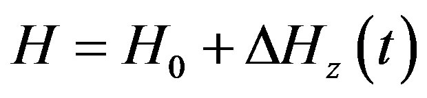
In order to give the description of spin in a non-static external field, let us consider the simplest case first. We now consider the form it takes for a spin of 1/2. First look at the most simple situation; there is a static external field in the z direction and plus an oscillating field in the x direction. The interaction energy between the spin magnetic moment and the field is.
 (1)
(1)
where ,
,  is the external field in the z direction and the Hamiltonian operator of the system is
 (2)
(2)
Considering a system whose nuclei posses spin m. The corresponding eigen-function of the time independent Schrodinger equation is denoted by , the time dependent solution corresponding to a particular value of m is
 (3)
(3)
Thus the most general time dependent solution is:
 (4)
(4)
where the cm’s are complex constants. We may compute the expectation value of any observable by means of . For simplicity we consider a system whose nuclei posses spin 1/2. By using (2), we get:
 (5)
(5)
Now consider a magnetic field H1, which rotates at angular velocity wz, in addition to the static field H. The total field is then:
 (6)
(6)
We have the time dependent Schrödinger equation for a proton
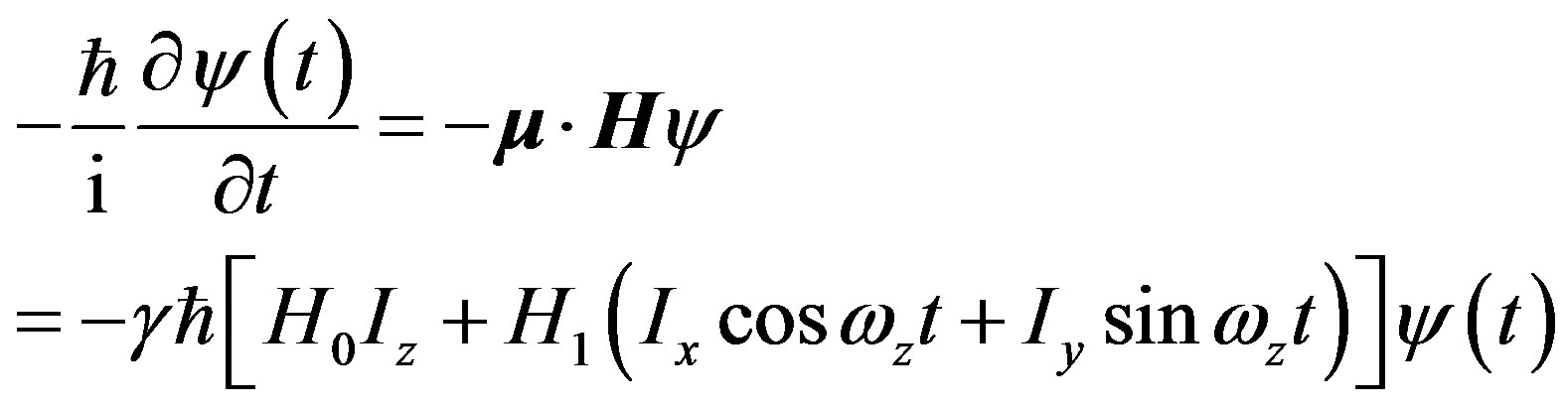 (7)
(7)
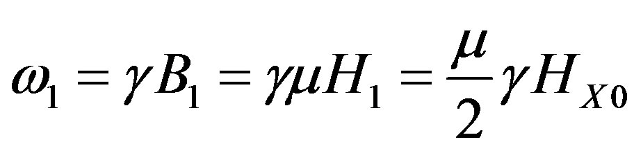
Let  (Larmor frequency). For a system whose nuclei posses spin 1/2, in the rotation coordinate system, it is convenient to express the wave function and the c’s in terms as follows:
 (8)
(8)
where  and
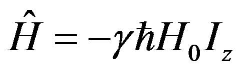
and  are the eigenstate of the spin operator Iz. Following discussion will focus on the case of a non-static external field that is the longitudinal magnetic field changes with time. Suppose when t = 0, the Hamiltonian operator of the system is:
 (9)
(9)
when , the resonance occurs in the system. However, the longitudinal magnetic field still has a change over time:
 (10)
(10)
In the rotation coordinate system effective magnetic field is not a static magnetic field [1], but a time dependent effective field
 (11)
(11)
when t > 0 , the Hamiltonian operator of the system is:
 (12)
(12)
In the rotation coordinate system, the Hamiltonian operator of the system is:
 (13)
(13)
And the time dependent Schrödinger equation become
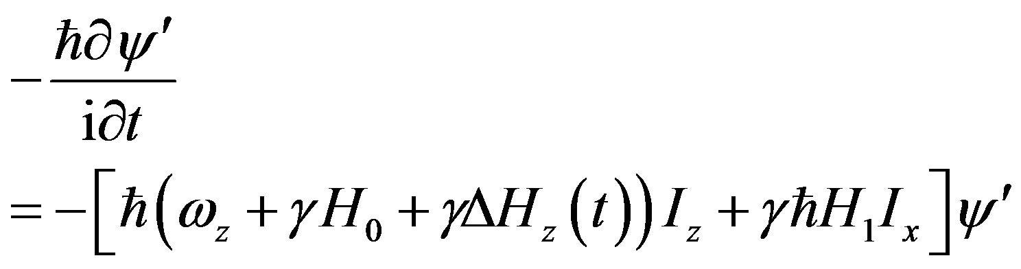 (14)
(14)
Take (8) into Schrödinger equation, we have
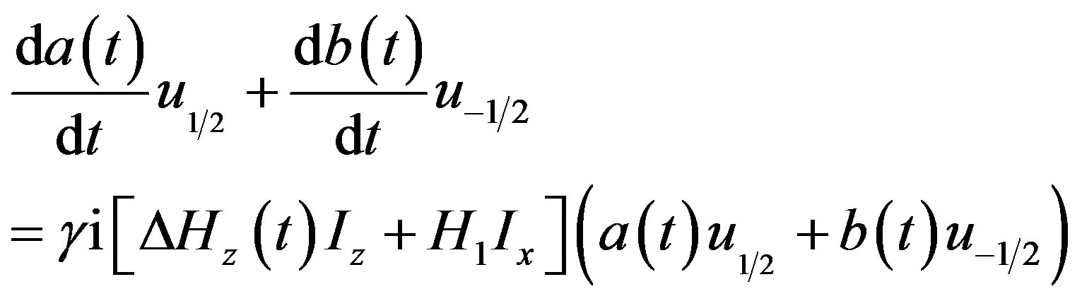 (15)
(15)
Multiplying by  from the left, integrating over spin space, the right side of the Equation (15) is:
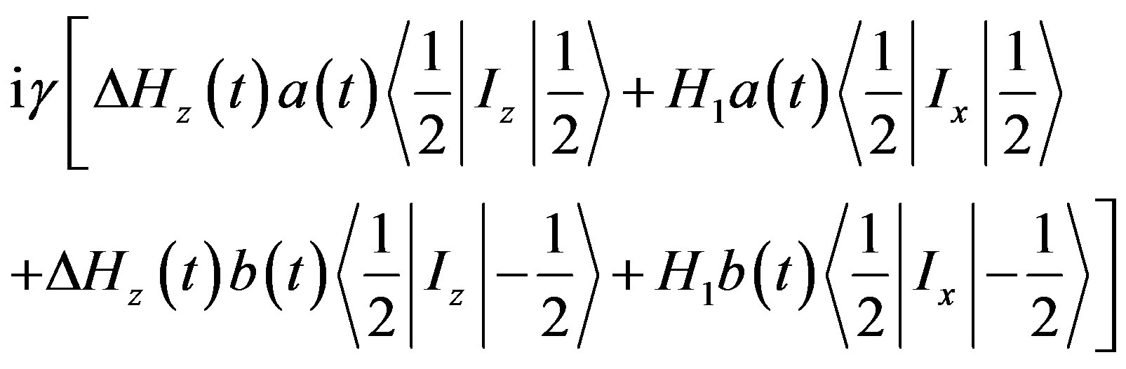 (16)
(16)
and consider the fact of that [1]:
 (17)
(17)
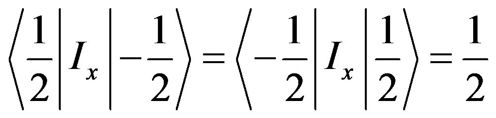 (18)
(18)
We get:
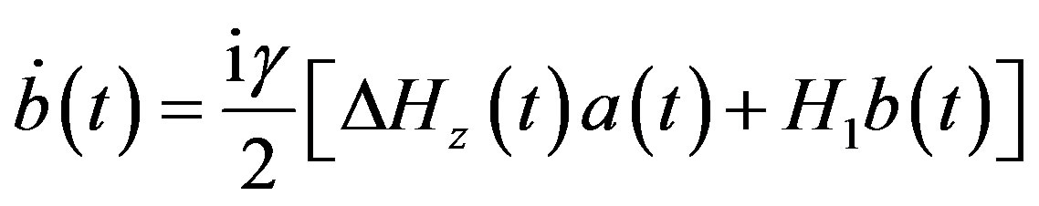 (19)
(19)
 (20)
(20)
Considering the rf pulse bandwidth is very short, within that time, the increment of the field can be approximated into a linear change over time: , (19) and (20) become:
 (21)
(21)
 (22)
(22)
Let ,
, , this is the precession frequency of the magnetic moment relative to x axis (relative to H1) in rotation coordinate system.
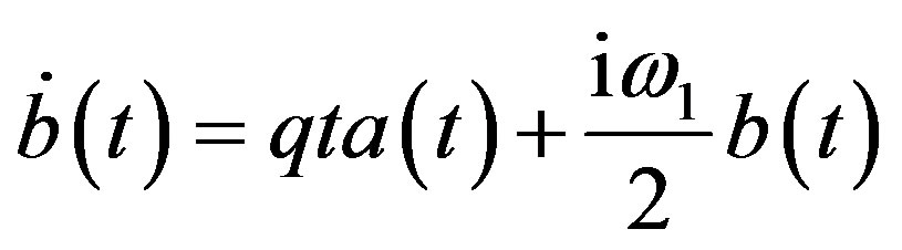 (23)
(23)
 (24)
(24)
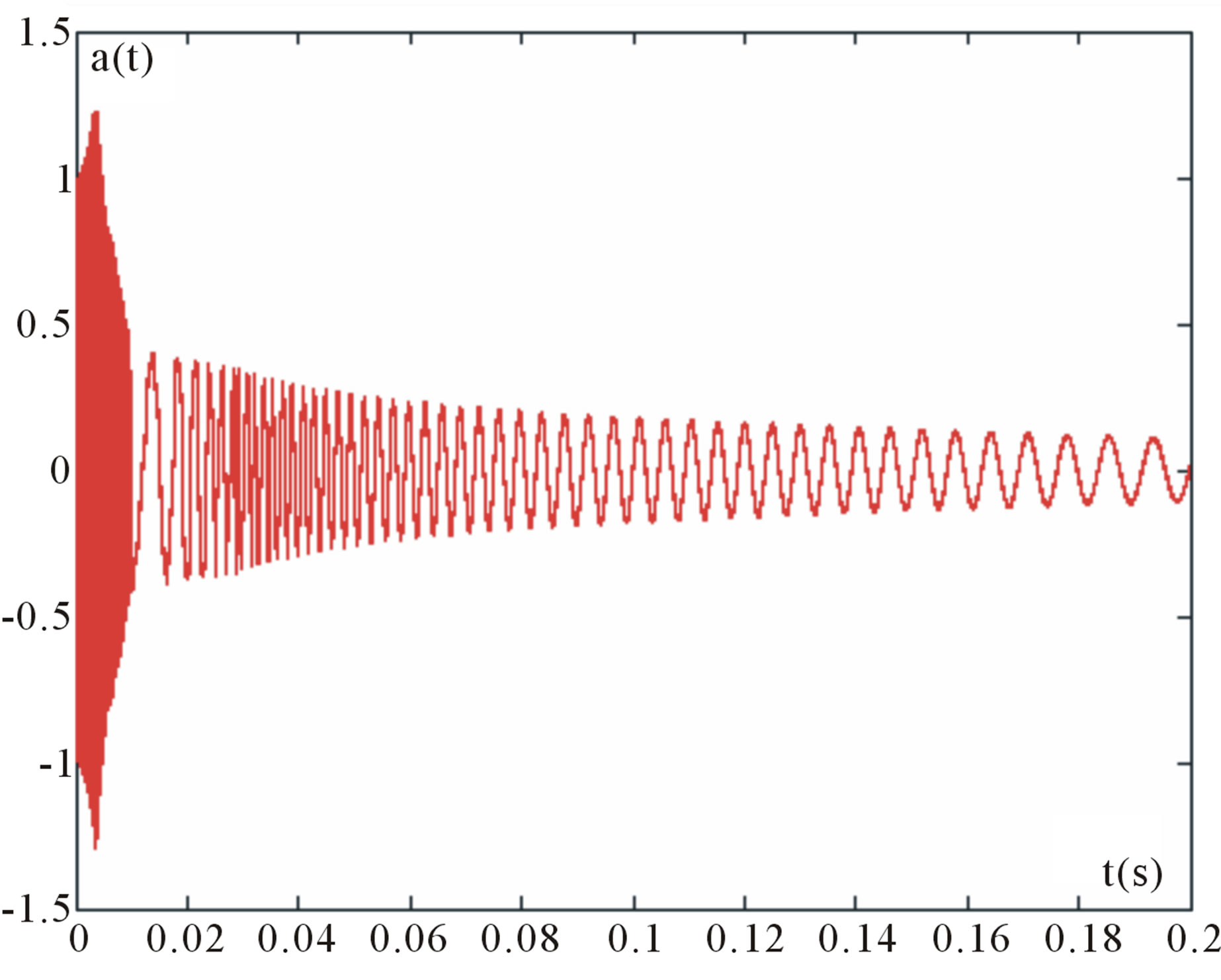
From a(t) and b(t), one can easily to determine the wave function by the Equation (8). Equations (23) and (24) are solved with Runge-Kutta method, and the solutions are shown in Figure 1.
3. The Susceptibility of the Sample in a Non Static Longitudinal Field
Considering that change rate over time of the vertical field is much slower than the transition speed of the quantum magnetic moment, so, quasi-static approximation can be used here. In other words, the orientations of the microscopic magnetic moments are quantized and the energy levels tend to comply with the Boltzmann distribution, at thermal equilibrium. Under local thermal equi-
 (a)
(a)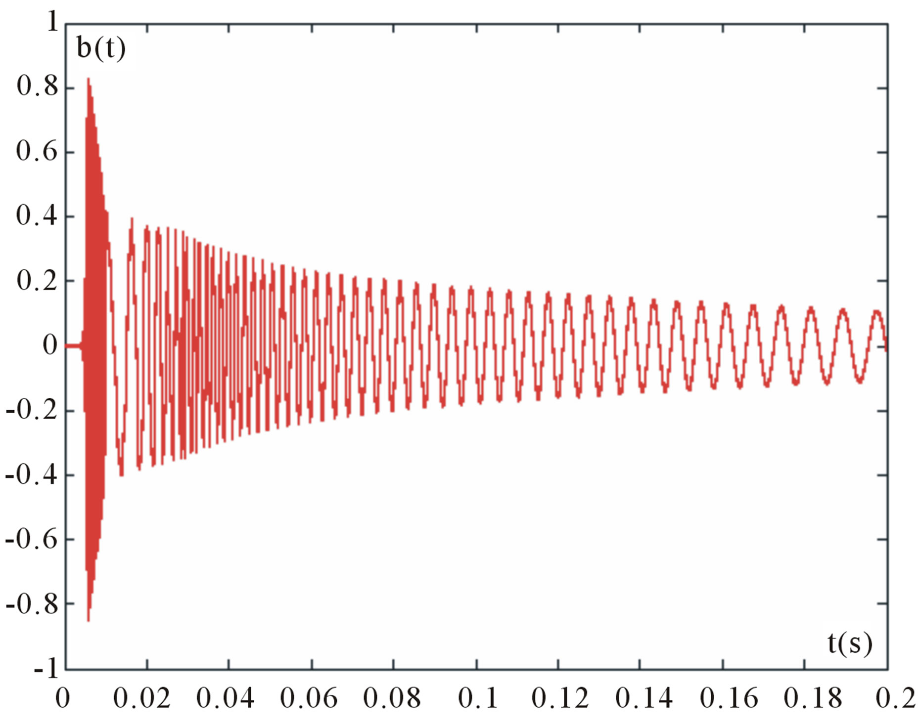 (b)
(b)
Figure 1. (a) The variation of a(t) with time; (b) The variation of b(t) with time.
librium hypothesis, the magnetization vector can be expressed as
 (25)
(25)
where I is the nuclear spin quantum number. According to electromagnetic theory
 (26)
(26)
Compare (25) and (26), magnetic susceptibility can be obtained:
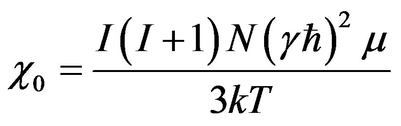 (27)
(27)
where m is permeability. In the non-ferromagnetic materials, we have m » m0.
In the case of macroscopic samples, unlike precession or nutation of a single magnetic moment in a magnetic field, the interaction among spin and the surrounding lattice, spin and spin must be considered, and it involves the spin—lattice relaxation and spin—spin relaxation, corresponding to T1 (longitudinal relaxation) and T2 (longitudinal relaxation). In this case, Bloch equation is the equation of motion of the macroscopic magnetization vector M [1],
 (28)
(28)
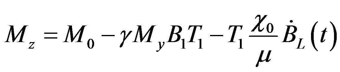
where  is the macro moment of samples at the moment of the transverse RF magnetic is added.
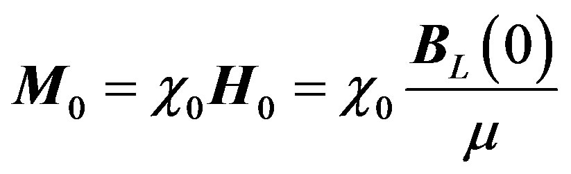 (29)
(29)
In the rotating frame of reference, RF field is constant, therefore
 (30)
(30)
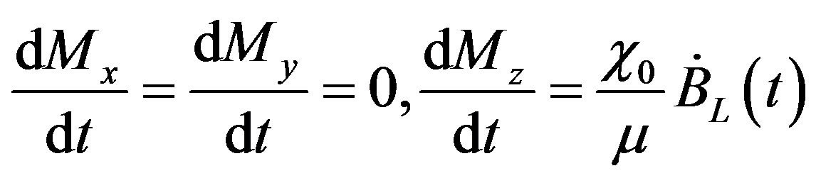
By the first equation in (28):
 (31)
(31)
Let
 (32)
(32)
 (33)
(33)
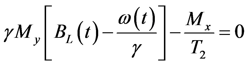
By the third equation in (28):
 (34)
(34)
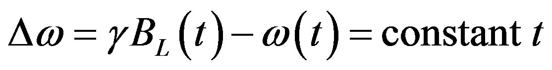
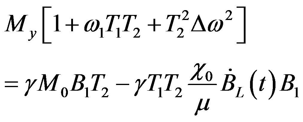
Take (34) into the second equation in (28), and let , we have
 (35)
(35)
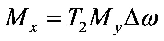
We get,
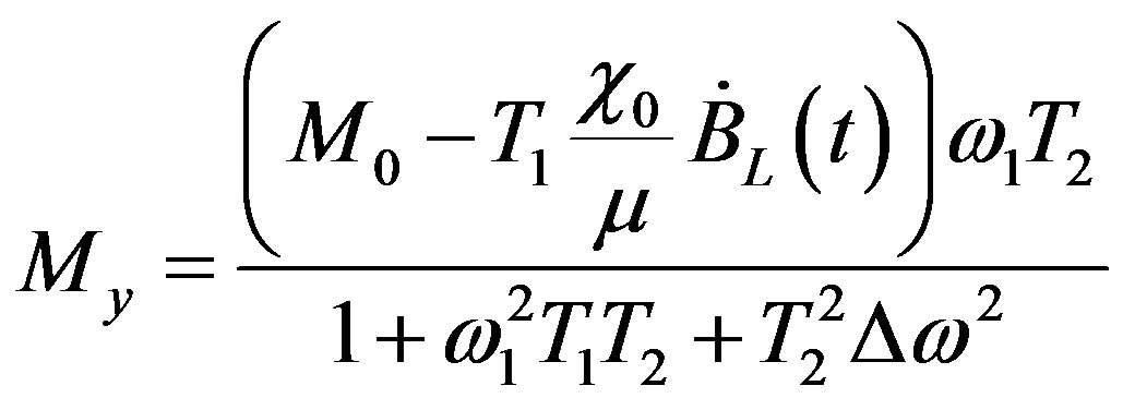 (36)
(36)
 (37)
(37)
Above result is acquired in rotating c frame of reference. Now considering the laboratory frame of reference, the magnetization vector of the sample can be expressed as
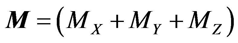 (38)
(38)
Here
 (39)
(39)
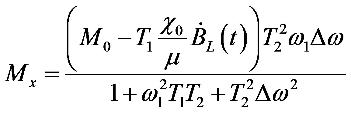
Take (36) and (37) into (39):
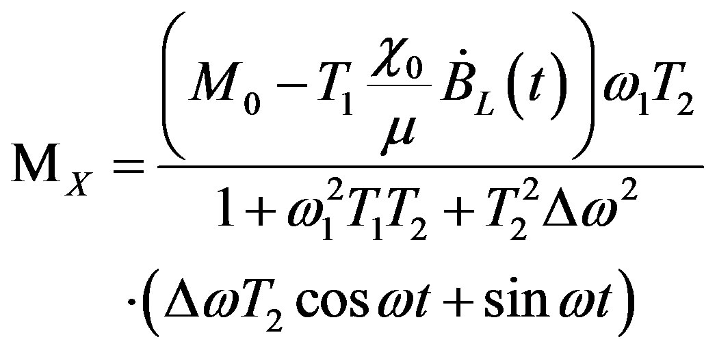 (40)
(40)
The RF field, BX0coswt, is expressed as superposition of levorotatory and dextral rotating fields, therefore
 (41)
(41)
and writing
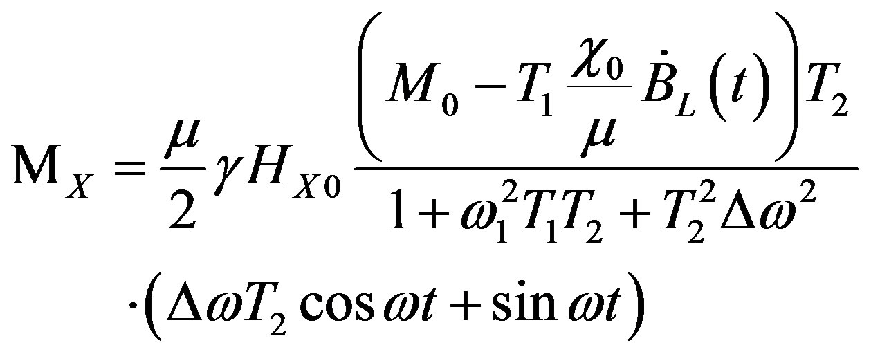 (42)
(42)
Compare (41) and (42), we find the plural dynamic susceptibility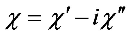 . The real and imaginary part can be written as
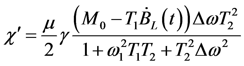 (43)
(43)
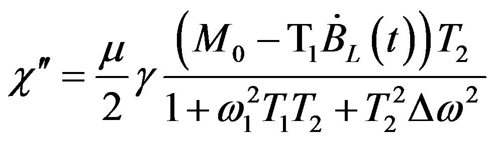 (44)
(44)
The effects of larmor precession frequency corresponding to the longitudinal field,  and rate of change of the longitudinal field are shown in Figure 2. In this calculation, we take m » m0;
  = 2.6752E4 and M0 = 0.03773 A/m, respectively.
According to the theory of the electric and magnetic fields, c’reflects the absorption of the sample to the alternating field, and 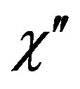 reflects the chromatic dispersion of the sample. From Figure 1, one can find that if the longitudinal field changes too fast, the chromatic dispersion of the sample become increase significantly and reduce the SNR (Signal-to-Noise Ratio). When the larmor frequency corresponding to the longitudinal field is
 (a)
(a) (b)
(b)
Figure 2. (a) The value of c′ versus Dw and variation rate of the longitudinal field; (b) The value of –c″ versus Dw and variation rate of the longitudinal field.
higher than the frequency of the RF field,  is positive, it means the inductance of the detecting coil become larger, while, if the larmor frequency corresponding to the longitudinal field is lower than the frequency of the RF field,
  is negative, it means the the inductance of the detecting coil become smaller. On the other hands, from Figure 2, one can find that when the frequency difference is small and as the longitudinal field changes rate increasing, the absorption of the sample become increase significantly, which is in favor of enhancing output power.
4. Conclusions and Prospect
Through The NMR signals in a time dependent longitudinal field is sensitive to both of the variation rate and frequency difference between larmor frequency corresponding to the longitudinal field and the frequency of the RF field. Increasing the longitudinal field changes rate is a double-edged sword to the quality of NMR spectroscopy, because both of the chromatic dispersion and the absorption of the sample increase significantly as the variation rate increase. The chromatic dispersion can work to the disadvantage of the SNR (Signal-to-Noise Ratio), and the absorption of the sample increasing is beneficial to the signal output power.
5. Acknowledgements
This work was supported by the Natural Science Foundation of China (Grant No. 10975056)
REFERENCES
- C. P. Slichter, “Principles of Magnetic Resonance,” Springer, New York, 1996.
- J. Haase and G. V. M. Williams, “NMR and Electronic Inhomogeneity in Cuprate Superconductors,” Current Applied Physics, Vol. 6, No. 3, 2006, 293-295. doi:10.1016/j.cap.2005.11.002
- J. Haase, M. Kozlov, K. H.Muller, et al., “NMR in Pulsed High Magnetic Fields at 1.3 GHz,” Journal of Magnetism and Magnetic Materials, Vol. 290-291, No. 1, 2005, pp. 438-441. doi:10.1016/j.jmmm.2004.11.494
- B. K. Mikhail, H. Jurgen and B. Christoph, “56 T 1H NMR at 2.4 GHz in a Pulsed High-Field Magnet,” Solid State Nuclear Magnetic Resonance, Vol. 28, No. 1, 2005, pp. 64-67. doi:10.1016/j.ssnmr.2005.06.003
- J. Haasea, M. B. Kozlova, A. G. Webbb and B. Buchnera, “2 GHz 1H NMR in Pulsed Magnets,” Solid State Nuclear Magnetic Resonance, Vol. 27, 2005, pp. 206-208.
- K. Kodama, M. Takigawa, et al., “Magnetic Superstructure in the Two-Dimensional Quantum Antiferromagnet SrCu2(BO3)2,” Science, Vol. 298, No. 5592, 2002, pp. 395-399. doi:10.1126/science.1075045
- K. Atsushi and I. Shinji, “Ultra-Broadband NMR Probe: Numerical and Experimental Study of Transmission Line NMR Probe,” Journal of Magnetic Resonance, Vol. 162, No. 2, 2003, pp. 284-299. doi:10.1016/S1090-7807(03)00014-4