ABSTRACT

We generalize the previously considered cases of a harmonic oscillator subject to a random force (Brownian motion), or having random frequency, or random damping. We consider here a random mass which corresponds to an oscillator where the particles of the surrounding medium adhere to the oscillator for some (random) time after collision, thereby changing the oscillator mass. Such a model is appropriate to chemical and biological solutions as well as to some nano-technological devices. The first moment and stability conditions for white and dichotomous noise are analyzed.

1. Introduction

Brownian motion is described by the dynamic equation of a harmonic oscillator supplemented by thermal noise

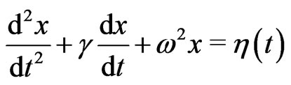(1)

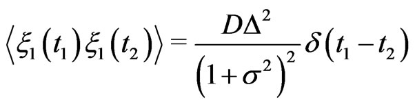
with the correlation function

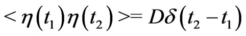(2)

The random force enters Equation (1) additively. When the noise has an external origin rather than an internal origin, the associated noise enters the equation of motion multiplicatively. If the noise arises from the fluctuations of the potential energy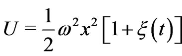the equation of motion (1) takes the following form

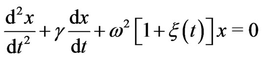(3)

Another possibility for the generalization of the dynamic Equation (1) is the inclusion of random damping

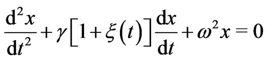(4)

There are many applications in physics, chemistry and biology of the models described by equations (3) and (4) [1].

We recently studied [2] still another possibility for introducing randomness in the oscillator Equation (1), by considering an oscillator with a random mass, which describes a new type of Brownian motion-Brownian motion with adhesion. In this situation the molecules of the surrounding medium not only randomly collide with the Brownian particle, which produces its well-known zigzag motion, but they also stick to the Brownian particle for some (random) time, thereby changing its mass. The appropriate equation of motion has the following form

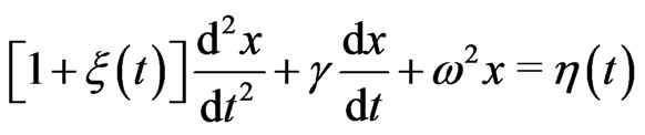(5)

Among applications of (5) is an RLC electrical circuit subject to a voltage with a fluctuating inductance which is described by the following equation

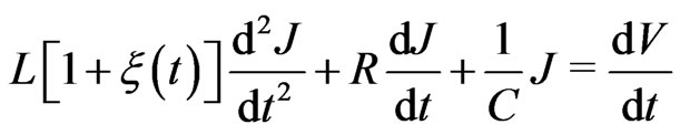(6)

There are many situations in which chemical and biological solutions contain small particles which not only collide with a large particle, but they may also adhere to it. The diffusion of clusters with randomly growing masses has also been considered [3]. There are also some applications of a variable-mass oscillator [4]. Modern applications of such a model include a nanomechanical resonator which randomly absorbs and desorbs molecules [5]. The aim of this note is to describe a general and simplified form of the theory of an oscillator with a random mass, which is a useful model for describing different phenomena in Nature.

2. Model

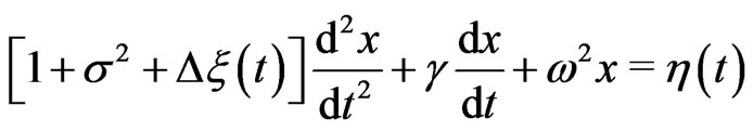
We have to modify Equation (5) slightly since this equation describes the dynamic equation with a mass that can both increase or decrease due to fluctuations. As distinct from Equations (3) and (4), we replace in Equation (5) by a positive random force which corresponds to the fact that the mass of the Brownian particle can only increase due to the adhesion of the molecules of the surrounding medium,

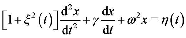(7)

We consider the simple form of color noise—the asymmetric dichotomous noise (random telegraphic process), which means that the random variable takes values or Denote the rate of transition for to by, and the reverse rate by. For this form of the Ornstein-Uhlenbeck noise, the correlation function is

(8)

For the limiting case of white noise, and with remaining constant,

(9)

The quadratic noise can be written as

(10)

with and Indeed, for, one obtains, and for

Equation (7) then takes the following form,

(11)

3. First Moment

First of all, one has to transfer the stochastic Equation (11) to the deterministic equations for the average values etc. For this purpose we use the well-known Shapiro-Loginov procedure [6] which yields for exponentially correlated noise (8)

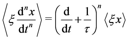(12)

Inserting (12) into (11) (with) one obtains, after averaging,

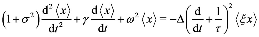(13)

A new function enters Equation (13). A second equation for the two functions and can be obtained by multiplying Equation (11) by

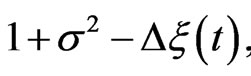
using Equation (12) and the following exact expression for the exponentially correlated noise, for splitting averages [7]

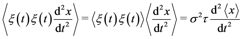(14)

which gives

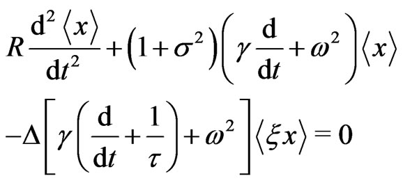(15)

where It was assumed that there is no correlation between the internal and external sources of noise,.

The advantage of dichotomous noise is that the averaging procedure (14) allows one to avoid an infinite system of high-order correlations. Excluding the correlator from Equations (13) and (15), one obtains a cumbersome fourth-order differential equation for which we do not write here. In a similar way one can find the equations for the second moment

4. Stability Conditions

Here we consider the much less trivial problem of the stability of the solutions. For a deterministic equation, the stability of the fixed points is defined by the sign of, found from the solution of the form of a linearized equation near the fixed points. The situation is quite different for a stochastic equation. The first moment and higher moments become unstable for some values of the parameters. However, the usual linear stability analysis, which leads to instability thresholds, turns out to be different for different moments making them unsuitable for the stability analysis. A rigorous mathematical analysis of random dynamic systems shows [8] that, similar to the order-deterministic chaos transition in nonlinear deterministic equations, the stability of a stochastic differential equation is defined by the sign of Lyapunov exponents. This means that for stability analysis, one has to go from the Langevin-type Equations (3), (4) and (11) to the associated FokkerPlanck equations which describe properties of statistical ensembles.

The Lyapunov exponent is defined as the exponential divergence rate of neighboring trajectories [8], i.e., as

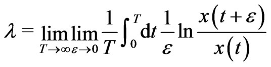(16)

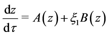
It is convenient to take limit first. Then, after substituting in (16) the expansion 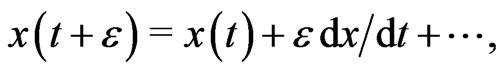one obtains

(17)

where the new variable has been introducedand is the stationary solution of the FokkerPlanck equations corresponded to the Langevin equations expressed in the variableTurning from the variable in the Langevin Equations (5), (6) and (11) to the variable one gets

(18)

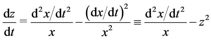
Multiplying Equation (11) with by one obtains

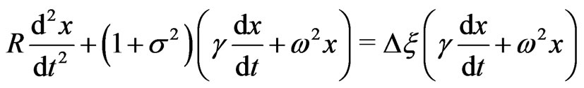(19)

Replacing the variable by the variable leads to

(20)

where

(21)

4.1. White Noise

First, we start with white noise for which

(22)

The Fokker-Planck equation associated with Equation (5) has the following form ( Stratonovich interpretation) [9]

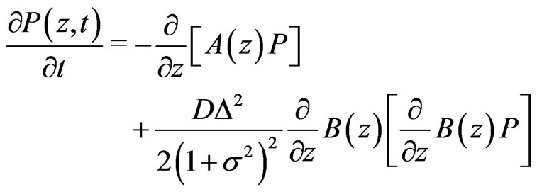(23)

which, for the stationary case reduces to

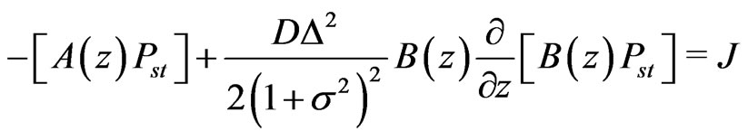(24)

where is the constant probability current.

The solution of the homogeneous Equation (24) (with) is

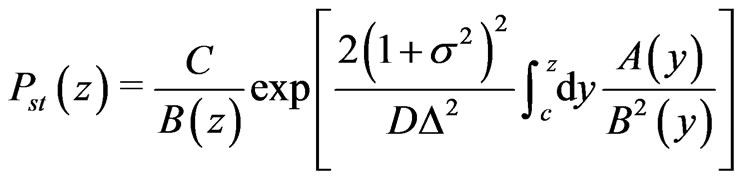(25)

The solution of the inhomogeneous Equation (24) can be obtained by the method of variation of constants, which leads to

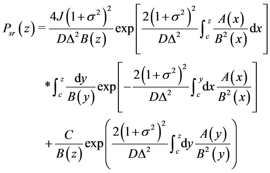(26)

The constant and the reference point are not important for our analysis, and we may assume for

Inserting (21) into (26), one transforms Equation (26) to the following form,

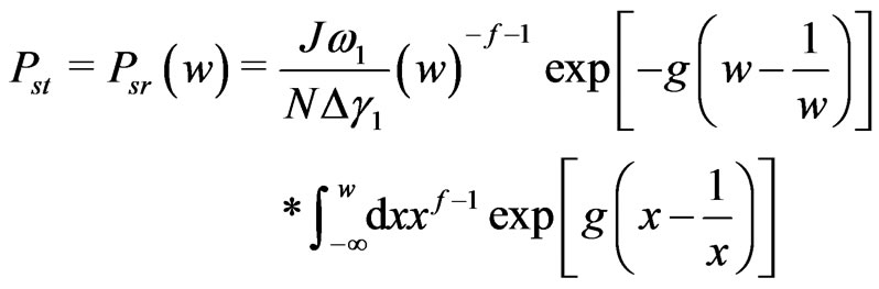(27)

where

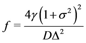(28)

There is no need to perform an analysis of Equation (27), since the analogous calculation has been performed for the case of random damping [10] yielding the following result after substitution in Equation (17),

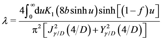(29)

where is a modified Bessel function of the second kind, and and are Bessel functions of the first and second kind, respectively. The Bessel functions are always positive, and the sign of the Lyapunov exponent is the same as the sign of the hyperbolic function, i.e., the sign of

Therefore, an oscillator with fluctuating mass becomes unstable when i.e., the instability of the fixed point occurs for 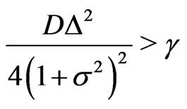and does not depend on the oscillator frequency.

4.2. Dichotomous Noise

According to [11,12], the stationary solution of the Fokker-Planck equation, corresponding to the Langevin Equation (19) having the correlation function (8), has the following form

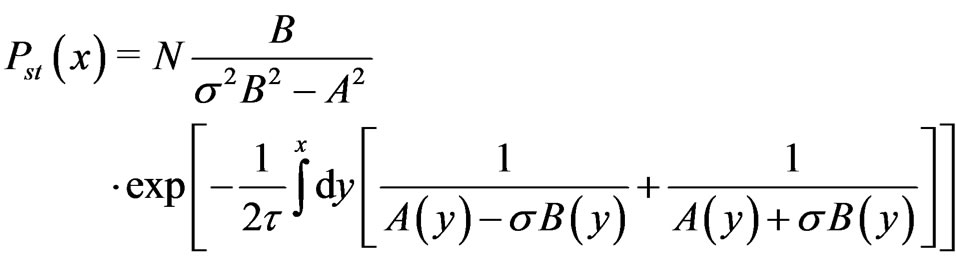(30)

Equation (30) has been analyzed for different forms of functions and:

[13]; [14] ;

[15];, [16];

[17,18]; [11,12].

The zeroes of functions determine the boundary of which diverges or vanishes at the boundaries and determine the boundary of support of The latter means that a system will approach the state located in intervals or depending on its initial position. Another important characteristic of is location of its extrema, which define the macroscopic steady states. The steady states of (30) obey the following equation [11,12].

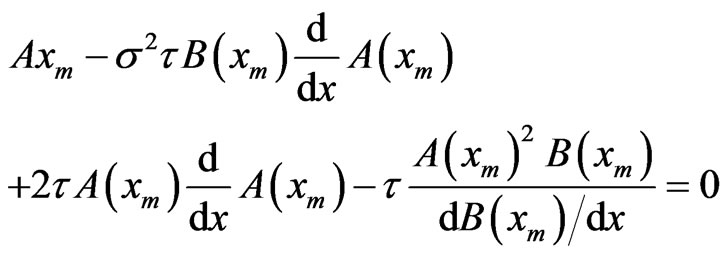(31)

The first term in (31) defines the deterministic steady states while the first two terms relate to the white noise limit (with 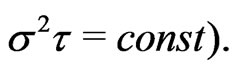Finally, the last two terms define the corrections coming from the final correlation time

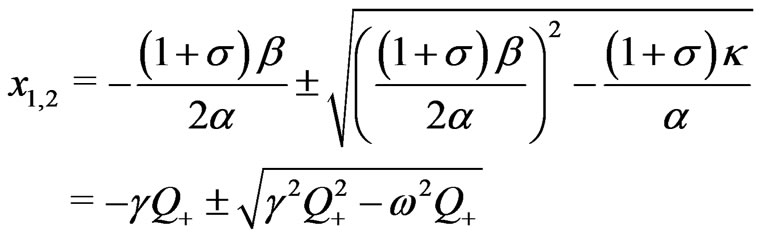
For

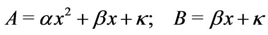(32)

with, according to (21),

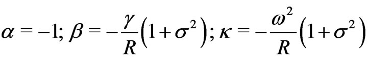(33)

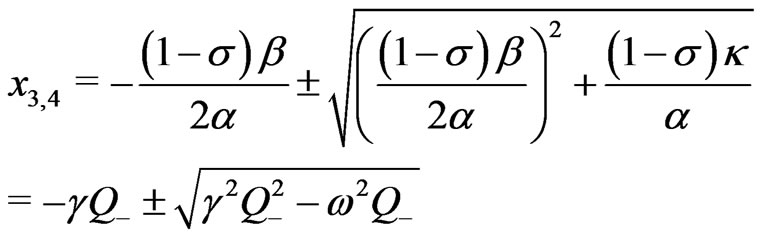
one obtains

(34)

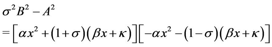
and

(35)

(36)

where

(37)

(38)

with

(39)

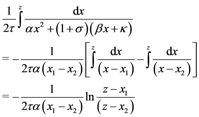
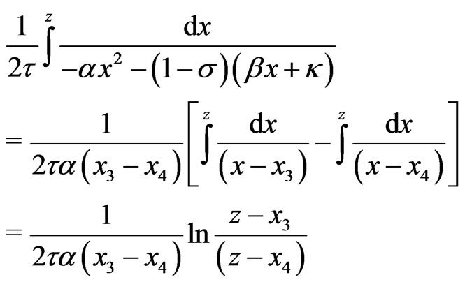
Inserting (32)-(38) into (30) gives

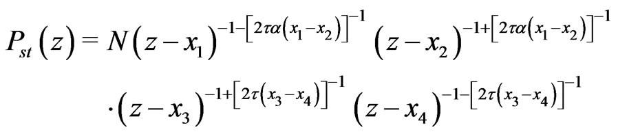(40)

which, according to (17), defines the boundary of stability of the fixed point for different values of parameters and, which depend on characteristics of an oscillator and and of noise.

5. Conclusions

We have introduced a new model of a stochastic oscillator having a fluctuating mass, which, among other processes, describes Brownian motion with adhesion. That is, the particles of the surrounding medium not only collide with the Brownian particle but also adhere to it for some (random) time after the collision, thereby changing its mass. For white and dichotomous sources of noise, one can find the two first moments. A detailed stability analysis has been performed for white and dichotomous noise.

REFERENCES

- M. Gitterman, “The Noisy Oscillator: the First Hundred Years, from Einstein until Now,” World Scientific, Singapore, 2005.
- M. Gitterman, “New Stochastic Equation for a Harmonic Oscillator: Brownian Motion with Adhesion,” Journal of Physics C, Vol. 280, 2010, p. 012049
- J. Luczka, P. Hanggi and A. Gadomski, “Diffusion of Clusters with Randomly Growing Masses,” Physical Review E, Vol. 51, No. 6, 1995, pp. 5762-5769.
- M. S. Abdalla, “Time-Dependent Harmonic Oscillator with Variable Mass under the Action of a Driving Force,” Physical Review A, Vol. 34, No. 6, 1986, pp. 4598-4605. doi:10.1103/PhysRevA.34.4598
- J. Portman, M. Khasin, S. W. Shaw and M. I. Dykman, “The Spectrum of an Oscillator with Fluctuating Mass and Nanomechanical Mass Sensing,” Bulletin of the American Physical Society, March Meeting 2010, Vol. 55, No. 2, Portland, 15-19 March 2010, Abstract V14.00010.
- V. E. Shapiro and V. M. Loginov, “Formula of Differentiation and Their Use for Solving Stochastic Equation,” Physica A, Vol. 91, No. 3-4, 1978, pp. 563-574. doi:10.1016/0378-4371(78)90198-X
- R. C. Bourret, U. Frish and A. Pouquet, “Brownian Motion of Harmonic Oscillator with Stochastic Frequency,” Physica A, Vol. 65, No. 2, 1973, pp. 303-320.
- L. Arnold, “Random Dynamic Systems,” Springer, Berlin, 1998.
- N. G. van Kampen, “Stochastic Processes in Physics and Chemistry,” Elsevier, North-Holland, 1992.
- N. Leprovost, S. Aumaitre and K. Mallick, “Stability of a Nonlinear Oscillator with Random Damping,” European Physical Journal, Vol. 49, 2006, pp. 453-458.
- K. Kitahara, W. Horsthemke and R. Lefever, “ColoredNoise Induced Transitions: Exact Results for External Dichotomous Markovian Noise,” Physics Letters A, Vol. 70, 1979, pp. 377-380.
- K. Kitahara, W. Horsthemke and R. Lefever, “Phase Diagrams of Noise Induced Transitions,” Progress Theoretical Physics, Vol. 64, 1980, pp. 1233-1247. doi:10.1143/PTP.64.1233
- V. I. Klyatskin, “Dynamic Systems with Parameter Fluctuations of the Telegraphic Process Types,” Radiophysics and Quantum Electronics, Vol. 20, 1977, pp. 384-393. doi:10.1007/BF01033925
- V. Berdichevsky and M. Gitterman, “Stochastic Resonance in Linear Systems Subject to Multiplicative and Additive Noise,” Physical Review E, Vol. 60, No. 2, 1999, pp. 1494-1499.
- F. Sasagawa, “Critical Slowing Dawn in Random Growing-Rate Models with General Two Level Markovian Noise,” Progress Theoretical Physics, Vol. 69, No. 3, 1983, pp. 790-800. doi:10.1143/PTP.69.790
- K. Ouchi, T. Horita and H. Fujisaka, “Critical Dynamics of Phase Transition Driven by Dichotomous Markov Noise,” Physical Review E, Vol. 74, 2006, p. 031106. doi:10.1103/PhysRevE.74.031106
- Y. Jia, X.-P. Zheng, X.-M. Hu and J.-R. Li, “Effect of Colored Noise in Stochastic Resonance in a Bistable System Subject to Multiplicative and Additive Noise,” Physical Review E, Vol. 63, 2001, p. 031107. doi:10.1103/PhysRevE.63.031107
- S. Z. Ke, D. J. Wu and L. Cao, “Phase Transitions in a Bistable System Driven by Two Colored Noise,” European Physical Journal B, Vol. 12, 1999, pp. 119-122. doi:10.1007/s100510050985