Applied Mathematics
Vol.10 No.03(2019), Article ID:91456,19 pages
10.4236/am.2019.103011
One-Dimensional Explicit Tolesa Numerical Scheme for Solving First Order Hyperbolic Equations and Its Application to Macroscopic Traffic Flow Model
Tolesa Hundesa1, Legesse Lemecha2, Purnachandra Rao Koya1
1School of Mathematical and Statistical Sciences, Hawassa University, Hawassa, Ethiopia
2Department of Mathematics, Adama Science and Technology University, Adama, Ethiopia

Copyright © 2019 by author(s) and Scientific Research Publishing Inc.
This work is licensed under the Creative Commons Attribution International License (CC BY 4.0).
http://creativecommons.org/licenses/by/4.0/


Received: January 10, 2019; Accepted: March 25, 2019; Published: March 28, 2019
ABSTRACT
In this paper, a new numerical scheme for solving first-order hyperbolic partial differential equations is proposed and is implemented in the simulation study of macroscopic traffic flow model with constant velocity and linear velocity-density relationship. Macroscopic traffic flow model is first developed by Lighthill Whitham and Richards (LWR) and used to study traffic flow by collective variables such as flow rate, velocity and density. The LWR model is treated as an initial value problem and its numerical simulations are presented using numerical schemes. A variety of numerical schemes are available in literature to solve first order hyperbolic equations. Of these the well-known ones include one-dimensional explicit: Upwind, Downwind, FTCS, and Lax-Friedrichs schemes. Having been studied carefully the space and time mesh sizes, and the patterns of all these schemes, a new scheme has been developed and named as one-dimensional explicit Tolesa numerical scheme. Tolesa numerical scheme is one of the conditionally stable and highest rates of convergence schemes. All the said numerical schemes are applied to solve advection equation pertaining traffic flows. Also the one-dimensional explicit Tolesa numerical scheme is another alternative numerical scheme to solve advection equation and apply to traffic flows model like other well-known one-dimensional explicit schemes. The effect of density of cars on the overall interactions of the vehicles along a given length of the highway and time are investigated. Graphical representations of density profile, velocity profile, flux profile, and in general the fundamental diagrams of vehicles on the highway with different time levels are illustrated. These concepts and results have been arranged systematically in this paper.
Keywords:
Hyperbolic Equation, Advection Equation, Tolesa Numerical Scheme, Traffic Flow, Numerical Simulation

1. Introduction
Hyperbolic partial differential equation of conservation laws has recently received great attention and many books have been published in this area [1] [2] [3] [4] . Hyperbolic PDEs describe the time dependent physical systems and can be used to model a wide variety of phenomenon including wave motion and advection transport of substances [5] . Advection equations do form a special class of conservative first order hyperbolic PDEs which transport a given property across a system at a specified rate. In advecting equations, the temporal and spatial derivatives of the conserved quantity are proportional to each other. That is . Thus, the advection equation for the function will be
(1)
In (1), the quantity v is a proportional constant and can be interpreted as the velocity along x-direction [6] . However, if then the characteristics are directed to the positive direction or to the right and if then they are directed to the negative direction or to the left. In other words the sign of v indicates the direction of propagation of information. In fact the advection Equation (1) is also called as the one-way wave equation and in this context v represents the speed of propagation of the wave. The advection Equation (1) admits general analytic solutions and representing respectively a wave motion along positive and negative x-directions. The lines in the plane on which is constant are called characteristics. The parameter v has dimensions of distance divided by time and is called the speed of propagation along the characteristic. We give at the initial time, is required to be equal to a given function or for all . This is called an initial value problem. Advection Equation (1) is being numerically solved using various one-dimensional explicit numerical schemes, for example Upwind, Downwind, FTCS and Lax-Friedrichs schemes. In these one-dimensional explicit schemes the space and time mesh sizes are restricted both by order of accuracy and numerical stability. The said schemes have been visualized with the unique schematic diagrams which are illustrated in Figures 1-4.
Having been studied carefully the space and time mesh sizes and patterns or schematic diagrams of all these schemes, another but a new scheme has been developed and named as one-dimensional explicit Tolesa numerical scheme. This new scheme has been visualized with the unique schematic diagram and is illustrated in Figure 5. The implication of the advection Equation (1) together with initial value problem in the context of Lighthill Whitham and Richards (LWR) traffic flow model is implemented. The LWR model is the well-known model and describes the traffic flow using a partial differential equation based on the conservation law of the vehicles in traffic [7] [8] [9] [10] . In this study, the single lane traffic flow with constant speed and linear density-speed relationship are considered as a test case. The simulations of traffic flow model with constant speed will also be done by using the mentioned one-dimensional explicit numerical schemes including Tolesa scheme, and linear density-speed relationship will be simulated by using Tolesa scheme.
In this research work we present and discuss some of the one-dimensional explicit numerical schemes available in the literature and the newly propose scheme. Specifically, the paper is organized in three more sections that follow this Introduction. Section 2 is devoted to carry out finite difference method. The finite difference approximations of the first order hyperbolic partial differential equation using one-dimensional explicit numerical schemes are presented. Section 3 reports about macroscopic continuum traffic flow depend mainly on three quantities flux, speed and density, and present some cases for speed-density relationship. Finally section 4 deals with the numerical simulation. In this section, we present the discretization of the macroscopic continuum traffic flow model, specifically Lighthill-Whitham and Richards Traffic flow model presented in section 3, using finite difference schemes presented in Section 2.
2. Overviews of Finite Difference Method
In this study, it is mainly focused to carry out finite difference method (FDM). The FDM was introduced by Euler in 18th century and has been greatly regarded as the easiest method and widely used to solve simple geometrical problems [11] . The FDM is classically obtained by approximating the derivatives appearing in the partial differential equation by a Taylor expansion up to some given order which will give the order of the scheme. The application of FDM in solving a PDE is to transform a calculus problem into an algebraic problem by discretizing the continuous physical domain into a number of cells or intervals, and approximating the individual exact partial derivatives in the PDE by algebraic finite difference approximations.
Let the spatial and temporal domains be divided into N and M cells respectively. The index represents a grid point where spatial and temporal grids intersect. Here and . Thus, the discretization of space-time domain is assumed as and . The quantities and respectively denote the spatial and temporal step sizes. These are also known as the increments between two consecutive spatial and temporal nodes respectively.
Let the quantity denote an approximate value of the function at the grid point or space-time location . That is . Thus, the function can now be replaced with a discrete set of point-wise approximate values . These approximations are called the finite difference approximations. The finite difference approximations of the first order hyperbolic partial differential Equation (1) using one-dimensional explicit numerical schemes are presented in the following subsection.
One Dimensional Explicit Numerical Schemes
In this subsection, the one-dimensional explicit numerical schemes with Upwind, Downwind, FTCS and Lax-Friedrichs schemes including Tolesa scheme are presented to approximate the spatial and temporal partial derivatives of the advection Equation (1) in different views as shown in Figures 1-5. Also the orders of accuracy and numerical stability have been determined in which the space and time mesh sizes are restricted. The approximations and the schematic diagrams of the mentioned schemes are explained sequentially.
In one-dimensional explicit upwind scheme, the first order spatial and temporal partial derivatives are approximated respectively as and . In this view, the stencil is given as shown in Figure 1 and the approximations of the finite difference form of Equation (1) can be expressed as
(2)
The scheme (2) is a first order accurate in both space and time, . This scheme is stable if the condition is satisfied.
In one-dimensional explicit downwind scheme, the first order spatial and temporal partial derivative are approximated respectively as
and .
In view of this the finite difference approximations form of Equation (1) can be expressed as
(3)
Equation (3) is a first order accurate in both space and time . This scheme is unconditionally unstable.
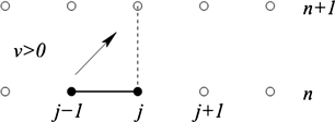
Figure 1. Stencil of One-dimensional explicit upwind numerical scheme.
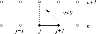
Figure 2.Stencil of one-dimensional explicit downwind scheme.
In one-dimensional explicit FTCS scheme, as its name implies, the first order temporal and spatial partial derivatives are obtained respectively by taking a first order forward finite differencing in time and a central differencing in space. These are approximated respectively as and . Then, the approximations of the finite difference form of Equation (1) can be expressed as in Equation (4) and the schematic diagram is given in Figure 3.
(4)
Equation (4) is a first order accurate in time and second order accurate in space, i.e., . This scheme is unconditionally unstable.
In one-dimensional explicit Lax-Friedrichs scheme, the term in FTCS scheme is replaced by its average value . In Lax-Friedrich scheme the finite difference form of Equation (1) can be expressed as (5) and its stencil is viewed as in Figure 4.
(5)
Equation (5) is a first order accurate in time and second order accurate in space, i.e., . This scheme is conditionally stable, if the condition is satisfied.
Having been studied carefully the space and time mesh sizes, and the patterns of all these schemes a new scheme has been developed and named as one-dimensional explicit Tolesa numerical scheme. The one-dimensional explicit Tolesa numerical scheme is still another alternative numerical scheme to solve advection equation and can be applied to traffic flows model. The schematic diagram of Tolesa evolution scheme is shown in Figure 5 and the application of this scheme to the advection Equation (1) is straightforward. In view of this, the first order temporal and spatial partial derivatives are approximated respectively as Equations (6) and (7).
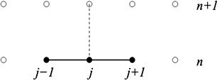
Figure 3. Stencil of one-dimensional explicit FTCS scheme.

Figure 4. Stencil of one-dimensional explicit Lax-Friedrichs scheme.

Figure 5. Stencil of one-dimensional explicit Tolesa scheme.
(6)
(7)
Let the term on the left hand side of (6) be expressed as the average value as
(8)
In (8), the terms on the left hand side can be expanded, as in view of (5), as
(9)
(10)
Using the three expansions (8)-(10) in the two Equations (6)-(7) and on substituting them in (1), the advection equation reduces to the form as
(11)
Here in (11), the notation is used. Thus, (11) is the newly proposed one-dimensional explicit Tolesa scheme. Equation (11) is a first order accurate in time and second order accurate in space, .
Local Truncation Error Local truncation error represents the difference between an exact differential equation and its finite difference representation at a point in space and time. Local truncation error provides a basis for comparing local accuracies of various difference schemes. Accordingly the local truncation error for Tolesa scheme (11) will be
by using Taylor’s expansion. Therefore, Tolesa scheme is first-order in time and second-order in space.
The fundamental properties that every finite difference approximation of a partial differential equation should possess are consistency, convergence and stability.
Consistence: The notion of consistency addresses the problem of whether the finite difference approximation is really representing the partial differential equation. We say that a finite difference approximation is consistent with a differential equation if the finite difference equations converge to the original equation as the time and space grids are refined. Hence, if the truncation error goes to zero as time and space grids are refined we conclude that the scheme is consistent. For the explicit solution to the advection equation, the truncation error is,
,
where
.
Thus as and , then , hence the Tolesa scheme is consistent with partial differential Equation (1) as long as .
Stability Analysis: A finite difference scheme is stable if the scheme do not allows the growth of error in the solution with different time level. Stability analysis is a useful tool for checking validity of a given numerical scheme [12] . There are many approaches to analyze whether a finite difference scheme is stable or unstable. In this paper, we will consider the Von Neumann stability analysis for presented finite difference schemes. The basic idea of this analysis is given by defining the discrete Fourier transform of u as (12). Let it be assumed that the solution can be seen as eigenmodes [13] which at each grid point have the form
(12)
Here in (12), is a complex number dependent on p and it works as an amplification factor; p is a real spatial wave number; is an imaginary number. Equation (12) shows the time dependence of a single eigenmode. The differential equations are said to be stable if .
Also, the Courant-Friedrichs-Lewy CFL criteria for stability say that if and only if . CFL is necessary condition for stability [14] .
Substituting (12) in (11) and solving the expression for is obtained:
From Von-Neumann stability analysis, Tolesa method is stable when .
After some computations, and considering different cases which satisfy equality and the CFL condition, then we decided that the .
(13)
Thus, the explicit Tolesa scheme is conditionally stable (13).
Convergence: A numerical scheme is convergent if the computed solution of the discretized equation leads to the exact solution of the differential equation as the time and grid spacing lead to zero. The computed solution must approach the exact solution of the differential equation at any point and when and lead to zero while keeping and constant. In other hand, the error
satisfying the following convergence condition.
, at fixed and . Hence, the explicit Tolesa scheme is convergent; we can see this from the simulations result.
3. Lighthill-Whitham and Richards Traffic Flow Model (LWR Model)
In this section, macroscopic continuum traffic flow model is introduced and analyzed. Macroscopic continuum traffic flow depends mainly on three quantities: traffic density, traffic flow or flux and traffic velocity [15] . The number of vehicles on a highway per unit length is defined as traffic density and is denoted by . The traffic flow rate or flux is defined as the number of vehicles passing through a given point x at time t and is denoted by . Here and . In this study, highway is considered as a unidirectional roadway of finite length with no entrances and exits.
The well-known Lighthill-Whitham and Richards (LWR) model describes the traffic flow using a partial differential equation constructed based on the conservation law of the vehicles in traffic. In this model the traffic flow is represented using a first order hyperbolic partial differential equation and is put as
(14)
The flux can also be expressed in terms of the traffic density and the traffic speed as
(15)
In view of (15), the traffic flow model (14) with initial condition takes the form as
(16)
Equation (16) is called an initial value problem IVP of the macroscopic traffic flow model.
In this study, Equation (16) has been considered in two different cases depending on the speed-density relationship as constant speed, and linear speed-density relationship. Also assuming that traffic flux and speed are expressed as a function of density and respectively.
Case 1: In this case Equation (16) can be expressed as (17) by considering constant speed v and the flux as a function of density .
(17)
The analytical solution of the form (17) has been calculated using the method of characteristics in implicit form [16] as follows.
(18)
Case 2: Linear speed-density function in 1935, Greenshields [17] proposed what was perhaps the first traffic flow model. According to his observations made using photographic methods, Greenshields postulated that there existed a linear relationship between speed and density. Then traffic flux . In this case Equation (16) can be expressed as
(19)
The analytical solution of the form (19) has been calculated using the method of characteristics in implicit form as follows.
(20)
4. Numerical Simulations
In this subsection, we present the discretization of the traffic flow model (17) using finite difference schemes (2)-(5), and (11) as shown in table below:
4.1. Traffic Flow with Constant Speed
In order to better understand, methods for highway design, it is necessary to discretize the given model using the numerical schemes and perform numerical experiments. The numerical discretization of traffic flow model using explicit finite difference schemes are shown in Table 1.
The numerical schemes given in Table 1 are implemented using the following

Table 1. Discretization of traffic flow model using explicit finite difference schemes, where the parameters and are used to represent the expressions and .
assumptions and values:
1) Highway is considered as a single lane of length 20 km. Thus .
2) The initial density of vehicles in this study is taken as in [18] , and from this the exact solution becomes .
3) The boundary condition is considered as constants: .
4) The total time duration is divided into 100 steps: .
5) The total spatial distance is divided into 100 steps: .
6) Vehicles are considered to flow with constant speed .
7) The temporal and spatial step lengths are considered as and .
Using these assumptions and the discretization shown in Table 1, we have developed computer programs to conduct simulation study of traffic flow model with constant velocity (17). Numerical experiments are performed on a time scale of 7 minutes and some qualitative behaviors of the schemes are verified. The simulation of the exact solution as in Figure 6(a) and numerical approximations of each schemes are shown in (Figure 6(b), Figures 6(d)-(f) and Figure 6(h)). The blue colored curves represent the density at 0.7th min; green colored represent the density at 3.5th min; red colors represent the density after 7th min.
In Figure 6, the plots are obtained using the exact solution and the discretized one-dimensional explicit numerical schemes in Table 1. All the schemes are implemented to show the traffic densitie profiles at 0.7, 3.5, and 7 minutes as shown in Figure 6. The Upwind, Lax-Friedrichs, and Tolesa schemes are conditionally stable, . That is, stable if and only if the physical velocity v is not bigger than the spreading velocity of the numerical schemes or if the condition is satisfied. Equavelently the time step must be smaller than the time taken for the vehicle to travel the distance of the spatial step . The amplitude of the wave increases as the Courant number increseases. But, does not blow up as far as the Courant number is satisfied. In all schemes as shown in (Figure 6(b), Figure 6(f), Figure 6(h)) of


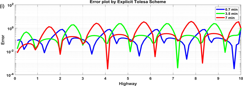
Figure 6. The plots of density profiles and numerical errors of the traffic flow model with constant speed at different time scales using the one-dimensional explicit numerical schemes. (a) The exact solution of the density profile; (b) The density profiles by Upwind scheme; (c) Error plot by Upwind scheme; (d) The density profiles by Downwind scheme; (e) The density profiles by FTCS scheme; (f) The density profiles by Lax-Friedrichs scheme; (g) Error by Lax-Friedrichs scheme; (h) The density profiles by Tolesa scheme; (i) Error plot by Tolesa scheme.
density profiles account lesser densities as time scale increase in comparison with those of the exact solution.
The downwind and FTCS schemes are unconditionally unstable as shown in (Figure 6(d), Figure 6(e)). The numerical scheme is unconditionally unstable indecating that the numerical solution will be destroyed by numerical errors which will be certainly produced and grow exponentially. That means, exponentially growing modes appear, rapidly destroying the solution. The amplitude of the wave strongly blow up or peak up and violate the numerical solution this is unphysical as shown in (Figure 6(d), Figure 6(e)).
(Figure 6(c), Figure 6(g), Figure 6(i)) indicate the numerical errors. The numerical errors increase as time scale increase. That is, the error formed at 7 min is larger than the error formed at 3.5 min and the error formed at 3.5 min is larger than the error formed at 0.7 min.
4.2. Traffic Flow with Linear Speed-Density Relationship
Greenshields proposed the first traffic flow model, and he observed that using photographic methods. The Greenshields was also able to show that a linear relationship between speed and density, and a quadratic relationship exists between flux and density, which, over the years, has come to be known as the fundamental diagram of traffic flow. In this subsection, we present the application of the Tolesa Scheme in the cases of traffic flow model with linear speed-density relationship as shown in Table 2. The LWR model (14) has been discretized by explicit Tolesa Scheme as follow.
The Tolesa scheme discretization given in Table 2 can be implemented using the same assumptions and values are used as in the case traffic flow model with
Table 2. Discretization of traffic flow model using explicit Tolesa schemes.
constant speed. Using these assumptions and the discretization shown in Table 2, we have developed computer programs to conduct simulation study of traffic flow model with linear density-speed relationship (19).
The exact solutions vary with location but almost the same for time as shown in Figure 7(a). The numerical errors increase as time scale increase. The error varies with time and location as shown in Figure 7(b). That is, the error formed at 7 min is larger than the error formed at 3.5 min and the error formed at 3.5 min is larger than the error formed at 0.35 min. The density, speed, and flow vary with time and location. As shown in Figures 7(c)-(e) Tolesa scheme is the correct simulation which express the reality and Mathematical relation between density, speed, and flow. An increase in density results in a decrease of vehicle speed and vehicle flow.
Fundamental Diagrams of Traffic Flow: Traffic flow theory involves the development of mathematical relationships among the primary elements of a traffic stream flow, density and speed. These relationships help traffic engineer in planning, designing, and evaluating the effectiveness of implementing traffic engineering measures on a highway system. Mathematical algorithms are used to study the complex interrelationship between elements of traffic stream. The diagrams shown in the relationship between speed-flow, speed-density, and flow-density are called the fundamental diagrams of traffic flow. These are as shown in Figure 10. The fundamental diagrams of traffic flow are vital tools which enables analysis of fundamental relationships. There are three diagrams: speed-density, speed-flow and flow-density.
1) Speed vs. Density: The variation of speed with density is linear as shown by the solid line in Figure 8. When there are no vehicles on the highway, the density is zero. When density is zero there will be little or no interaction between vehicles, therefore drivers are free to travel at max possible speed. Further continuous increase in density will then result in continuous reduction of speed,

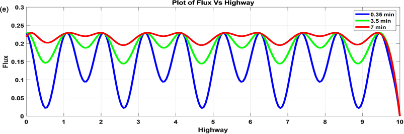
Figure 7. The plots of density profiles and numerical errors of the traffic flow modeat different time scales using the one-dimensional explicit numerical schemes. (a) Exact solution of the density profiles; (b) Error plot for linear density-speed relationship by Tolesa scheme; (c) Density profiles by Tolesa scheme; (d) Speed profiles by Tolesa scheme; (e) Flux profiles by Tolesa scheme.

Figure 8. Speed-density linear relationship by Tolesa scheme.
which will be zero when density is equal to the jam density. The maximum speed will be referred to as the free flow speed, and when the density is maximum, the speed will be zero.
2) Flow vs. Density: At zero density, the flow is obviously zero, because there are no vehicles on the road. As the density begins to rise, so does the flow, until a maximum flow is achieved at a critical density. Up to this point the movement of vehicles is relatively free and there is little interaction between the vehicles. An increase in density results in a decrease of vehicle speed and vehicle flow; this continues up to jam density, when traffic comes to a standstill. The flow and density varies with time and location. The relation between the density and the corresponding flow on a given stretch of road is referred to as one of the fundamental diagram of traffic flow and shown in Figure 9.
3) Speed vs. Flow: When flow is very low, there is little interaction between vehicles, therefore drivers are free to travel at max possible speed. The absolute max speed is obtained as the flow tends to zero. A point will be reached when further addition of vehicles will result in the reduction in the actual number of vehicles that pass a point on the highway (reduction of flow). At this point congestion is reached and eventually both speed and flow become zero. The flow is zero either because there are no vehicles or there are too many vehicles so that they cannot move. At maximum flow, the speed will be in between zero and free flow speed. The maximum flow occurs at critical speed. It is possible to have two different speeds for a given flow. The relationship between the speed and flow is referred to as one of the fundamental diagram of traffic flow and shown in Figure 10.
5. Conclusion
In the present work, one-dimensional explicit Tolesa scheme is developed for solving advection Equation (1) and is successfully applied on macroscopic traffic flow model with constant velocity (17). The one-dimensional explicit Tolesa
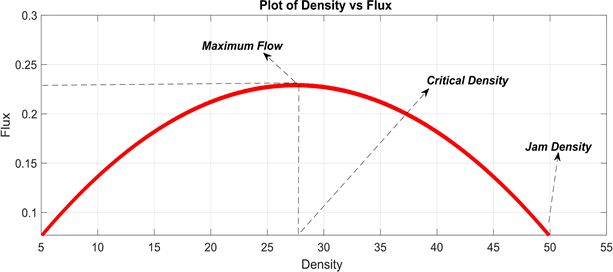
Figure 9. Density-flux nonlinear relationship by Tolesa scheme.
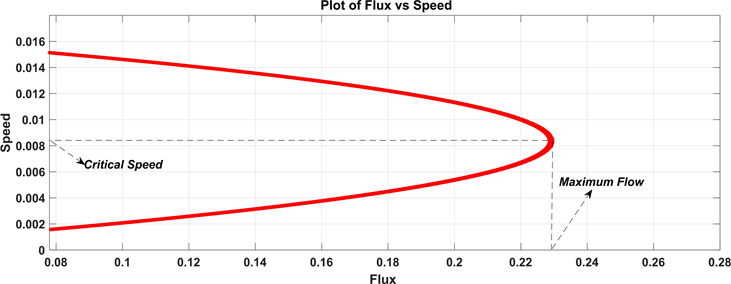
Figure 10. Flux-speed nonlinear relationship by Tolesa scheme.
numerical scheme is another alternative numerical scheme to solve advection equation and apply to traffic flows model like other well-known one-dimensional explicit schemes such as Upwind, Downwind, FTCS, and Lax-Friedrichs schemes. The one-dimensional explicit Tolesa Scheme has unique schematic diagram as others one-dimensional explicit Schemes. One-dimensional explicit Tolesa scheme is conditionally stable by Von Neumann stability analysis. Although the Tolesa scheme has been developed to find a numerical solution of advection equation, traffic flow with constant speed, and linear density-speed relationship, it can also be extended for first and second order traffic flow models with non-linear velocity-density relationships. The further applications of Tolesa scheme will be taken up in the further study.
Acknowledgements
This research work was supported by the Hawassa University and Wolaita Sodo University under the Ministry of Education. The contents of this paper reflect the views of the authors contributed equally to prepare, develop and carry out this manuscript.
Conflicts of Interest
The authors declare no conflicts of interest regarding the publication of this paper.
Cite this paper
Hundesa, T., Lemecha, L. and Koya, P.R. (2019) One- Dimensional Explicit Tolesa Numerical Scheme for Solving First Order Hyperbolic Equations and Its Application to Macroscopic Traffic Flow Model. Applied Mathematics, 10, 119-137. https://doi.org/10.4236/am.2019.103011
References
- 1. Quarteroni, A. (2009) Numerical Models for Differential Problems. Modeling, Simulation and Applications, Springer-Verlang, Milan, Vol. 2, 325-354.
https://doi.org/10.1007/978-88-470-1071-0 - 2. Lakhouili, A., Essoufi, El., Medromi, H. and Mansouri, M. (2015) Numerical Simulation of Some Macroscopic Mathematical Models of Traffic Flow. Comparative Study. International Journal of Computer Science, 3, 1-6.
- 3. Hoffma, J.D. (2001) Numerical Methods for Engineers and Scientists. 2nd Edition, Marcel Dekker Inc., New York.
- 4. Elena Vázquez-Cendón, M. (2015) Solving Hyperbolic Equations with Finite Volume Methods. Springer International Publishing, Berlin, Vol. 90.
https://doi.org/10.1007/978-3-319-14784-0 - 5. Leveque, R.J. (202) Finite Volume Methods for Hyperbolic Problems. The Press Syndicate of the University of Cambridge, Cambridge.
- 6. Noye, J. (1981) Finite Difference Methods for Partial Differential Equations. In: Numerical Solutions of Partial Differential Equations, North-Holland Publishing Company, University of Adelaide South Australia, 9-21.
- 7. Afroz, A., Kabir, M.H. and Andallah, L.S. (2014) A Computational Study of the Non-Dimensional Two Lane Traffic Flow Model with Two Sided Boundary Conditions. American International Journal of Research in Science, Technology, Engineering & Mathematics, 8, 50-56.
- 8. Chronopoulos, A. (1992) Efficient Traffic Flow Simulation Computations. Mathematical and Computer Modelling, 16, 107-120.
https://doi.org/10.1016/0895-7177(92)90123-3 - 9. Kabir, M.H., Gani, M.O. and Andallah, L.S. (2010) Numerical Simulation of a Mathematical Traffic Flow Model Based on a Non-Linear Velocity-Density Function. Journal of Bangladesh Academy of Sciences, 34, 15-22.
https://doi.org/10.3329/jbas.v34i1.5488 - 10. Gani, M.O., Hossain, M.M. and Andallah, L.S. (2011) A Finite Difference Scheme for a Fluid Dynamic Traffic Flow Model Appended with Two-Point Boundary Condition. GANIT: Journal of Bangladesh Mathematical Society, 31, 43-52.
- 11. Ferziger, J.H. and Peric, M. (2002) Computational Methods for Fluid Dynamics. Springer, Berlin.
https://doi.org/10.1007/978-3-642-56026-2 - 12. Strikwerda, J.C. (2004) Finite Difference Schemes and Partial Differential Equations. Society for Industrial and Applied Mathematics, Philadelphia.
- 13. Rezzolla, L. (2011) Numerical Methods for the Solution of Partial Differential Equations. Albert Einstein Institute, Max-Planck Institute for Gravitational Physics, Potsdam.
- 14. Bressan, A. (2016) Research Themes on Traffic Flow on Networks.
- 15. Hasan, M., et al. (2015) Lax-Friedrich Scheme for the Numerical Simulation of a Traffic Flow Model Based on a Nonlinear Velocity Density Relation. American Journal of Computational Mathematics, 5, 186-194.
https://doi.org/10.4236/ajcm.2015.52015 - 16. Stavroulakis, I.P. and Tersian, S.A. (2004) Partial Differential Equations and an Introduction with Mathematica and Maple. 2nd Edition, World Scientific Publishing, Singapore, 130-140.
- 17. Greenshields, B., et al. (1935) A Study of Traffic Capacity. Highway Research Board Proceedings, 14, 448-477.
- 18. Ali, A. and Abdallah, L.S. (2016) Inflow Outflow Effect and Shock Wave Analysis in a Traffic Flow Simulation. American Journal of Computational Mathematics, 6, 55-65.
https://doi.org/10.4236/ajcm.2016.62007