Applied Mathematics
Vol.08 No.01(2017), Article ID:73792,20 pages
10.4236/am.2017.81006
Modeling Walking with an Inverted Pendulum Not Constrained to the Sagittal Plane. Numerical Simulations and Asymptotic Expansions
Guillermo H. Goldsztein
School of Mathematics, Georgia Institute of Technology, Atlanta, GA, USA

Copyright © 2017 by author and Scientific Research Publishing Inc.
This work is licensed under the Creative Commons Attribution International License (CC BY 4.0).
http://creativecommons.org/licenses/by/4.0/


Received: November 30, 2016; Accepted: January 21, 2017; Published: January 24, 2017
ABSTRACT
Inverted pendulum models are commonly used to study the bio-mechanics of biped walkers. In its simplest form, the inverted pendulum consists of a point mass attached to two straight mass-less legs. Most works constrain the motion of the mass to the sagittal plane, i.e. the plane perpendicular to the ground that contains the direction toward the biped is walking. In this article, we remove this constrain to study the oscillations, the mass experiences in the direction perpendicular to the sagittal plane as the biped walks. While small, these lateral oscillations are unavoidable and of importance in the understanding of balance and stability of walkers, as well as walkers induced oscillations in pedestrian bridges.
Keywords:
Mathematical Modeling, Inverted Pendulum, Mechanics of Walking, Sagittal Plane, Oscillations

1. Introduction
When a human walks, the sagittal plane refers to the plane perpendicular to the ground that contains the direction toward the person is walking. As the person walks, its center of mass oscillates, both in the vertical direction (perpendicular to the ground) and lateral direction (perpendicular to the sagittal plane). One of our goals is to contribute to the understanding of the lateral oscillations.
The lateral oscillations play an important role in the balance and stability of individuals as they walk. Thus, their understanding is of interest in the field of bio-mechanics. These oscillations are also of interest in the field of robotics, since their understanding and control are likely to help improve the design of stable biped robots. While small, these lateral oscillations are the cause of some observed undesired and unexpected motions of pedestrian bridges when too crowded [1] - [11] . Thus, the topic of study of this article is also of interest to those that design pedestrian bridges as well as other related structures.
The use of inverted pendulum models to study the bio-mechanics of walking is a common practice. In its simplest form, the inverted pendulum consists of a point mass, which models the center of mass of the individual, attached to two straight mass-less segments, the legs. Works that use inverted pendulum (in its simplest or more sophisticated forms) or similar models to study aspects of the mechanics of biped walkers or related toys or biped robots include [12] - [26] . Particularly, the work in [27] has inspired lots of subsequent work.
Different simple models are surveyed in [28] . Inverted pendulum type models are also used to study the control and stability of walking [29] [30] and the balance of standing in moving platforms [31] . Some general articles about biped and animal movement, including walking and running, are [32] [33] . Spring loaded inverted pendulum models refer to inverted pendulum models where the legs are not rigid; instead, they behave like springs. These models are used to study the mechanics of running [34] [35] [36] . Spring loaded inverted pendulum models have also been used to study the transition from walking to running as the speed increases [34] [35] [37] [38] [39] . A survey regarding the analysis and control of biped robots walking can be found in [40] . Experimental studies of the responses of humans walking in a treadmill subject to lateral oscillations are reported in [41] . Lateral stability of walking is studied both theoretically and experimentally in [42] [43] [44] [45] [46] . The relationship between width of the step and length of the leg is studied with a mathematical model and energy arguments in [47] .
Most works using the simplest inverted pendulum model constrain the motion of the center of mass to the sagittal plane. In this article, we remove this constrain. As a consequence, we are able to use this unconstrained inverted pendulum model to study the lateral oscillations the mass experiences as the person walks, i.e. the oscillations in the direction perpendicular to the sagittal plane. We believe and hope that the model and techniques described in this article will be adopted by other researchers and will prove useful in the study of different aspects of the mechanics of biped walkers.
In the next section the model is introduced. In the following section we describe the equations governing the dynamics of the mass while one foot is off the ground. Subsequently, we identify the solutions to the governing equations that correspond to periodic walking. We then report results of numerical simulations. We further explore our model by restricting our attention to the parameter regime of slow walkers. We then also study the short steps parameter regime. We finish the article with a discussion.
2. The Model
We model a human as a point mass attached to two straight mass-less segments, the legs. Each leg is of length . The mass is the common end point of the two legs. The other end point of each leg is its foot. Only the feet can touch the ground. We will call this model of a human the model biped. Next, we describe our modeling assumptions. In the statements below k is any integer.
Assumption 1. At all times, either one or both feet are touching the ground.
The fact that each step takes the same time leads to our next assumption.
Assumption 2. Let be the time of one step. Both feet are touching the ground only at times .
During the time interval , the foot of only one leg is touching the ground. This leg is called the stance leg. The other leg is called the swing leg. For definiteness, we assume the left and right leg alternate being the stance and swing legs as follows.
Assumption 3. The left leg is the stance leg during the time intervals and thus, the right leg is the stance leg during the time intervals .
Assumption 4. During the time interval , the foot of the stance leg remains in the same position.
Observation 1. During the time interval , the only forces acting on the mass are the force due to gravity, , and the force due to the stance leg, , which is parallel to the stance leg and points from the mass in the direction opposite to the foot (see Figure 1).
As it makes contact with the ground at time , the leg that was the swing leg during the time period exerts an impulse on the mass , changing its momentum, and preventing the mass from falling to the ground. Simultaneously, the leg that was the stance leg during the time period #Math_18#, exerts another impulse on the mass , changing its momentum further, and giving the mass enough energy to take its next step. This last impulse corresponds to the human pushing off the ground with the foot of the leg that is changing from being the stance leg to being the swing leg. The impulse each leg exerts on the mass must be parallel to that leg and pointing from the mass away from its foot. This discussion leads to the next assumption.
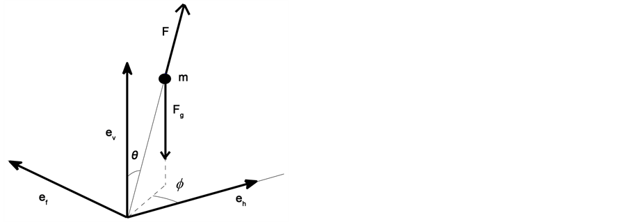
Figure 1. Forces acting on the mass . The stance leg is the solid thin line. The swing leg is not shown.
Assumption 5. Let , and denote the position of the mass and left and right foot at time respectively. At times , the mass feels an impulse of the form for some and , with and for all . By symmetry, we also have .
Observation 2. Since the legs and feet are mass-less, the motion of the swing leg does not affect the motion of the mass . It only matters the position where its foot lands.
Assumption 6. When both feet are touching the ground, at , the mass is in the plane that contains both feet and is perpendicular to the ground.
One could wonder if, when both feet are touching the ground, the mass could be out of the plane perpendicular to the ground containing the feet. An initial guess could lead us to believe that the mass being slightly ahead of this plane could facilitate the motion and make walking forward more efficient. However, in the context of this simple model, we have proved that there is no periodic walking if the mass is out of this plane. While elementary, this proof is somewhat tedious and lengthy, so we have elected to leave it out of this article.
In Figure 2 we illustrate and introduce geometric parameters. The solid circles are the footprints. The footprints from the left foot are included in a dotted line. The footprints from the right foot are included in the other dotted line. These two lines are a distance apart. Thus, models width of the steps. The white circles are the orthogonal projections onto the ground of the mass at times when both feet are touching the ground. After each step, the center of mass advances a distance . Thus, models the length of the steps. is the dimensionless unit vector that points in the direction the biped is walking. is the dimensionless unit vector perpendicular to , parallel to the ground and pointing to the right of the biped. is the dimensionless unit vector perpendicular to the ground pointing upward (see Figure 1 also).
Recall that is the time of one step and is the position of the mass at time . The symmetry and periodicity of the walk leads to the next assumption.
Assumption 7. for all . The components of the velocity of in the walking and vertical directions, and , are periodic with period and the component of the velocity of in the lateral direction, , is anti-periodic with anti-period .

Figure 2. Footprints, in solid black circles. The thin solid lines are the orthogonal projections of the legs onto the ground at the beginning and end of a step where the left leg is the stance leg.
3. Governing Equations during a Step While One Leg Is Off the Ground
We now proceed to describe the motion of the mass during the time interval . Recall that . During this period, the left leg is the stance leg and the right foot does not make contact with the ground. The left leg and the mass form an inverted pendulum. According to Observation 1 and Newton’s third law
(1)
where primes denote derivatives with respect to .
Let be the dimensionless unit vector pointing from the left foot to the mass, . We define , where is the acceleration of gravity and we use the notation for the norm of any vector , i.e. . We introduce the dimensionless time . Equation (1) becomes
(2)
where dots denote derivatives with respect to .
Let be the polar angle and be the azimuthal angle,
(3)
where and (see Figure 1). In terms of and , Equation (2) becomes
(4)
(5)
(6)
We will solve these equations during the first step, i.e. in the time interval , where . Equation (6) determines . The dynamics of the mass is given by Equations (4) and (5). Multiply Equation (5) by and integrate once to obtain
(7)
for some constant . Use Equation (7) to eliminate from Equation (4) to get . This equation is integrated once after is multiplied by to get
(8)
for some . Note that is the dimensionless mechanical energy.
The initial azimuthal angle, , and polar angle, , are related to the parameters displayed in Figure 2 (see also Figure 1). More precisely, let
(9)
then
(10)
Assume the parameters , and are given. For each pair #Math_106# and , the system of Equations (7) and (8) subjected to the initial conditions (9) and (10) has a unique solution. However, this solution may not correspond to periodic walking as described in this article. In the next section, we list the two necessary and sufficient conditions for periodic walking. These conditions will lead to a relationship between and .
4. Conditions for Periodic Walking
In this section we assume that the parameters , and are given and fixed. Thus, and are also given through Equations (9) and (10). We seek to answer the following question: Given that and , what are the necessary and sufficient conditions for periodic walking?
Condition 1. If and , solutions of Equations (7) and (8) subjected to the initial conditions (9) and (10), correspond to periodic walking, there exists such that and .
Note that is the dimensionless time of one step. simply means that the height of the mass at the start and the end of a step is the same. The need for is illustrated in Figure 2 and is a consequence of the symmetry of the steps.
Given any function of one variable, we use the standard notations and for the limits of as tends to from the right (with values of ) and from the left (with values of ). Given two vectors and we denote by their dot product.
Let be the unit vector from the left foot to the mass at time and let be the unit vector from the right foot to the mass at time . Given Assumption 7, if correspond to periodic walking. This fact, plus Assumption 5 leads to the second condition for periodic walking.
Condition 2. If and , solutions of Equations (7) and (8) subjected to the initial conditions (9) and (10), correspond to periodic walking, there exists
and such that .
In the above condition is as defined in Condition 1, and is related to and by Equation (3).
Observation 3. If Conditions 1 and 2 are necessary and sufficient for periodic walking.
Observation 4. If Condition 1 is satisfied, so is Condition 2.
The proof of this observation is simple. One shows that, if Condition 1 is satisfied, and for some positive constants and , from where we conclude that Condition 2 is satisfied with . The corresponding calculations are elementary but lengthy so we do not present them here.
The azimuthal angle initially decreases and it attains its minimum at the time such that . The value of this minimum azimuthal angle , can be obtained in terms of the constants of motion and from Equation (8) by setting
(11)
Note can be computed as follows
(12)
Due to symmetry, the Condition 1 is equivalent to: The minimum azimuthal angle is attained at the same time that the polar angle is zero, i.e.
. Thus, since , setting in Equation (12), using the fact
that , using Equations (7) and (8) and simple manipulations, we get that Condition 1 is satisfied if and only if
(13)
On one hand, given , Equation (8) implies that . On the other hand, we recall that the force the stance leg exerts on the mass points from the mass away from its foot. This means that in Equation (6) is constrained to be positive. Thus, while Equation (6) is not used to solve for and , it does impose a constrain. Using Equations (7) and (8) and simply algebra we get that . Thus, the constrain reduces to . Since is a decreasing function of for , this constrain needs to be verified only for . In summary, if the pair corresponds to periodic walking, we necessarily have . Note that the constrain gives a limit on the speed of the biped. If the biped were to try to walk faster, the foot of its stance leg would lose contact with the ground.
Since , we have that (see Equation (7)). On the other hand, given and , Equation (8) implies that the largest value of possible is the one that makes . Simple algebraic manipulations leads to the following constrain on once and are given, .
We summarize the findings in this section, and add to that, in the following observation.
Observation 5. (1) Let be given, the pairs that correspond to periodic walking are the solutions of Equations (11) and (13).
(2) If the pair corresponds to periodic walking, then and .
(3) Let be given. For each , there exist a such that , and the pair satisfies Equations (11) and (13) (we prove this point in Appendix 1).
(4) Let be given. Numerical simulations strongly suggest that, for each , there exist a unique such that , and the pair satisfies Equations (11) and (13) (i.e. the from point (3) is unique).
(5) While we were not able to prove it, we have evidence to believe that, if and , there is no periodic walking. Note that means that the feet are wider apart than the length of the steps, not a situation we will be considering. Thus, in the rest of this article, we will restrict our attention to the parameter regime and assume that
5. Numerical Simulations
In what follows we will study aspects of the periodic walking of the model biped. The parameters that determine the motion are , and . The angles and determine the geometry of the biped, i.e. the width and length of the steps relative to the length of the legs. The parameter is a dimensionless mechanical energy.
Let be the dimensionless time of one step. By symmetry, , the minimum azimuthal angle (see Equation (11)). Thus, . Using Equation (8) and simple manipulations we get
(14)
Let be the dimensionless average velocity. From Figure 2, it can be shown that the dimensionless distance the biped covers in one step is . Thus,
(15)
For the parameter values , Figure 3 shows as a function of . As expected, is an increasing function of . The more mechanical energy the mass has, the faster it moves in average. Our numerical calculations suggest that .
Let be the dimensionless amplitude of the lateral oscillations. Note that . Thus, from Equation (3) and the facts that and when , we have
(16)
Figure 3 shows as a function of when . Since increases with , note that is a decreasing function of . The faster the biped walks, the smaller the amplitude of the lateral oscillations.
Let be the dimensionless amplitude of the vertical oscillations. The mass is at its lowest when and its highest when . Thus, , which is
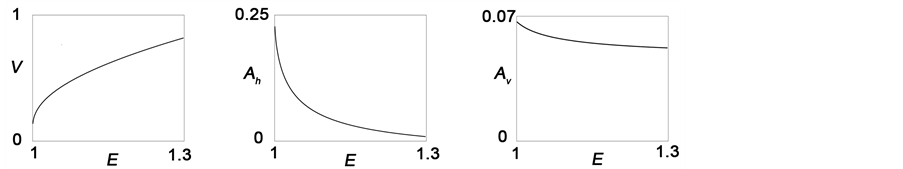
Figure 3. , and vs when .
(17)
With the parameter values , Figure 3 shows as a function of . Note that is a decreasing function of . The faster the biped moves, the smaller the vertical oscillations.
In Figure 4 we show an example of the path traced by the mass in two full steps. The top figure shows a three dimensional plot of the path of the mass. This path is the thick solid line. The thin lines are snapshots of the stance leg, the left leg during the first step and the right leg during the second step. The swing leg is not shown. The bottom figure shows a view from the top, i.e. the orthogonal projection of the path onto the ground. The lateral oscillations are clearly seen in this figure. Again, the thick solid line is the projection of the path of the mass and the thin lines are the projections of the stance leg. The parameters in that example are and .
6. Slow Walkers
We remind the reader that the dimensionless energy satisfies the constrains . In this section, we will study the dynamics of slow walkers. As our analysis will show, this corresponds to values of the energy of the form
(18)
The choice of the square in is to simplify future calculations. The fact that will allow us to use asymptotic approximations and as thus, obtain a deeper understanding of the dynamics of the model biped than by numerical simulations alone.
In the Appendix 2 we show that the asymptotic value of the minimum polar angle (see Equation (11)) valid in the parameter regime of Equation (18) is
(19)
In the Appendix 3 we show that the asymptotic value of the dimensionless time of one step, (see Equation (14)), is
(20)
In the above equation, we mean that . Thus, the dimensionless average velocity (see Equation (15)) satisfies, in this parameter regime
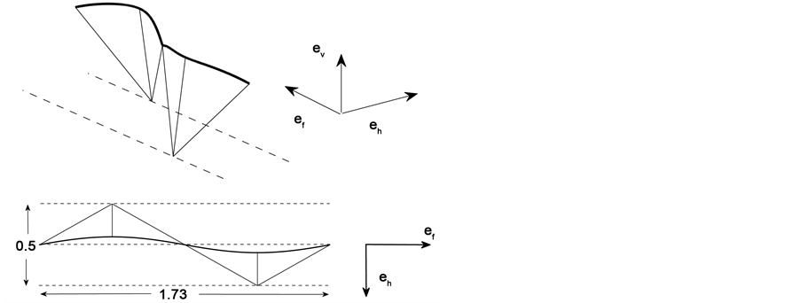
Figure 4. Trajectory of the mass . The value of the parameters are and .
(21)
Note that and as , consistent with the title of this section: slow walkers. Note also that the asymptotic formula for is consistent with the plot in Figure 3, not only on the fact that as (or ), but also on how it approaches 0.
Given Equation (19), we can obtain the asymptotic value of the amplitude of the lateral oscillations from Equation (16):
(22)
Figure 5 shows an example with the parameters are and . In this case, . We show the orthogonal projection of the trajectory of the mass onto the ground.
Compare Figure 5 with Figure 4, that was obtained with the same values of and but a value of , or in other words, . Note also that those two figures illustrate that the lateral oscillations increase as the velocity of the biped decreases.
7. Steps Much Shorter Than the Biped Height
In this section, we explore a different parameter regime. Namely, we restrict our attention to small values of the initial azimuthal angle
(23)
This corresponds to the biped taking steps that are much shorter than the lengths of its legs, a realistic parameter regime.
In the Appendix 4, we outline the steps required to get the asymptotic value of the minimum azimuthal angle and of in the regime . We obtain
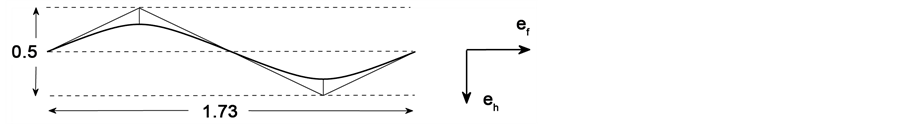
Figure 5. Orthogonal projection of the trajectory of the mass . The value of the parameters are and .
(24)
and
(25)
The asymptotic value of the dimensionless time required by the biped to take one step, , is obtained from Equations (14), (24) and (25) and simple manipulations
(26)
Thus, , the dimensionless average velocity of the biped satisfies
(27)
(see Equation (15)).
Making use of Equations (24) and (16) we get the asymptotic value of the amplitude of the lateral oscillations
(28)
Note that becomes small fast. It is of the order of for small values of .
On the other hand, the amplitude of vertical oscillations goes to zero quadratically as , since simple calculations lead to
(29)
Explicit Time Dependence of the Azimuthal Angle and Polar Angle When
As previously defined, is the dimensionless time required by the biped to take one step. Note that is a decreasing function of in the time interval . Thus, using Equation (8), the asymptotic value of (Equation (25)), the asymptotic approximations and when , and simple algebra we get
(30)
Using the initial conditions , this simple separable first order equation can be integrated analytically to get
#Math_334# (31)
On the other hand, Equation (7) leads to
(32)
Note that is given by Equation (31). Plugging that expression for as a function of into Equation (32), integrating, and using the initial condition , leads to the following formula
(33)
8. Discussion
In this article, we use a very simple inverted pendulum model to explore aspects of the mechanics of biped walkers. The novelty of this article is that we do not restrict the motion of the mass of the pendulum to the sagittal plane. As a consequence, we were able to study the lateral oscillations of the center of mass as the biped walks. These oscillations were beyond the capability of the simplest inverted pendulum models when the motion of the mass was restricted to the sagittal plane.
We performed numerical simulations and explore different parameter regimes with the use of asymptotic techniques. Our analysis shows that the inverted pendulum model remains simple enough to study, even when the mass is not restricted to move in the sagittal plane. We believe and hope the approach introduced in this paper will prove useful and be adopted by other researchers to study different aspects of the dynamic of biped walkers.
Cite this paper
Goldsztein, G.H. (2017) Modeling Walking with an Inverted Pendulum Not Constrained to the Sagittal Plane. Numerical Simulations and Asymptotic Expansions. Applied Mathematics, 8, 57-76. http://dx.doi.org/10.4236/am.2017.81006
References
- 1. Abdulrehem, M.M. and Ott, E. (2009) Low Dimensional Description of Pedestrian-Induced Oscillation of the Millennium Bridge. Chaos: An Interdisciplinary Journal of Nonlinear Science, 19, Article ID: 013129. https://doi.org/10.1063/1.3087434
- 2. Bachmann, H. (1992) Case Studies of Structures with Man-Induced Vibrations. Journal of Structural Engineering, 118, 631-647. https://doi.org/10.1061/(ASCE)0733-9445(1992)118:3(631)
- 3. Bocian, M., Macdonald, J.H.G. and Burn, J.F. (2012) Biomechanically Inspired Modelling of Pedestrian-Induced Forces on Laterally Oscillating Structures. Journal of Sound and Vibration, 331, 3914-3929. https://doi.org/10.1016/j.jsv.2012.03.023
- 4. Bodgi, J., Erlicher, S. and Argoul, P. (2007) Lateral Vibration of Footbridges under Crowd-Loading: Continuous Crowd Modeling Approach. Key Engineering Materials, 347, 685-690. https://doi.org/10.4028/ www.scientific.net/kem.347.685
- 5. Bruno, L., Venuti, F. and Nascé, V. (2012) Pedestrian-Induced Torsional Vibrations of Suspended Footbridges: Proposal and Evaluation of Vibration Countermeasures. Engineering Structures, 36, 228-238. https://doi.org/10.1016/j.engstruct.2011.12.012
- 6. Dallard, P., Fitzpatrick, T., Flint, A., Low, A., Smith, R.R., Willford, M. and Roche, M. (2001) London Millennium Bridge: Pedestrian-Induced Lateral Vibration. Journal of Bridge Engineering, 6, 412-417. https://doi.org/10.1061/(ASCE)1084-0702(2001)6:6(412)
- 7. Eckhardt, B., Ott, E., Strogatz, S.H., Abrams, D.M. and McRobie, A. (2007) Modeling Walker Synchronization on the Millennium Bridge. Physical Review-Series E, 75, Article ID: 021110. https://doi.org/10.1103/PhysRevE.75.021110
- 8. Ingólfsson, E.T., Georgakis, C.T., Ricciardelli, F. and Jonsson, J. (2011) Experimental Identification of Pedestrian-Induced Lateral Forces on Footbridges. Journal of Sound and Vibration, 330, 1265-1284. https://doi.org/10.1016/j.jsv.2010.09.034
- 9. Ingólfsson, E.T., Georgakis, C.T. and Jonsson, J. (2012) Pedestrian-Induced Lateral Vibrations of Footbridges: A Literature Review. Engineering Structures, 45, 21-52. https://doi.org/10.1016/j.engstruct.2012.05.038
- 10. Macdonald, J.H.G. (2008) Lateral Excitation of Bridges by Balancing Pedestrians. Proceedings of the Royal Society of London A: Mathematical, Physical and Engineering Sciences, 465, 1055-1073.
- 11. Venuti, F. and Bruno, L. (2009) Crowd-Structure Interaction in Lively Footbridges under Synchronous Lateral Excitation: A Literature Review. Physics of Life Reviews, 6, 176-206. https://doi.org/10.1016/j.plrev.2009.07.001
- 12. Adamczyk, P.G., Collins, S.H. and Kuo, A.D. (2006) The Advantages of a Rolling Foot in Human Walking. Journal of Experimental Biology, 209, 3953-3963. https://doi.org/10.1242/jeb.02455
- 13. Alexander, R.M. (1991) Energy-Saving Mechanisms in Walking and Running. Journal of Experimental Biology, 160, 55-69.
- 14. Alexander, R.M. (1992) A Model of Bipedal Locomotion on Compliant Legs. Philosophical Transactions of the Royal Society B: Biological Sciences, 338, 189-198. https://doi.org/10.1098/rstb.1992.0138
- 15. Coleman, M.J., Garcia, M., Mombaur, K. and Ruina, A. (2001) Prediction of Stable Walking for a Toy That Cannot Stand. Physical Review E, 64, Article ID: 022901. https://doi.org/10.1103/PhysRevE.64.022901
- 16. Coleman, M.J. and Ruina, A. (1998) An Uncontrolled Walking Toy That Cannot Stand Still. Physical Review Letters, 80, 3658. https://doi.org/10.1103/PhysRevLett.80.3658
- 17. Donelan, J.M., Kram, R. and Kuo, A.D. (2002) Simultaneous Positive and Negative External Mechanical Work in Human Walking. Journal of Biomechanics, 35, 117-124. https://doi.org/10.1016/S0021-9290(01)00169-5
- 18. Garcia, M., Chatterjee, A. and Ruina, A. (2000) Efficiency, Speed, and Scaling of Two-Dimensional Passive-Dynamic Walking. Dynamics and Stability of Systems, 15, 75-99. https://doi.org/10.1080/713603737
- 19. Garcia, M., Chatterjee, A., Ruina, A. and Coleman, M. (1998) The Simplest Walking Model: Stability, Complexity, and Scaling. Journal of Biomechanical Engineering, 120, 281-288. https://doi.org/10.1115/1.2798313
- 20. Geyer, H., Seyfarth, A. and Blickhan, R. (2006) Compliant Leg Behaviour Explains Basic Dynamics of Walking and Running. Proceedings of the Royal Society of London B: Biological Sciences, 273, 2861-2867. https://doi.org/10.1098/rspb.2006.3637
- 21. Goswami, A., Espiau, B. and Keramane, A. (1997) Limit Cycles in a Passive Compass Gait Biped and Passivity-Mimicking Control Laws. Autonomous Robots, 4, 273-286. https://doi.org/10.1023/A:1008844026298
- 22. Kuo, A.D. (2001) A Simple Model of Bipedal Walking Predicts the Preferred Speed-Step Length Relationship. Journal of Biomechanical Engineering, 123, 264-269. https://doi.org/10.1115/1.1372322
- 23. Kuo, A.D. (2002) Energetics of Actively Powered Locomotion Using the Simplest Walking Model. Journal of Biomechanical Engineering, 124, 113-120.
- 24. Kuo, A.D. (2007) The Six Determinants of Gait and the Inverted Pendulum Analogy: A Dynamic Walking Perspective. Human Movement Science, 26, 617-656. https://doi.org/10.1016/j.humov.2007.04.003
- 25. McGeer, T. (1993) Dynamics and Control of Bipedal Locomotion. Journal of Theoretical Biology, 163, 277-314. https://doi.org/10.1006/jtbi.1993.1121
- 26. Xiang, Y., Arora, J.S. and Abdel-Malek, K. (2010) Physics-Based Modeling and Simulation of Human Walking: A Review of Optimization-Based and Other Approaches. Structural and Multidisciplinary Optimization, 42, 1-23. https://doi.org/10.1007/s00158-010-0496-8
- 27. McGeer, T. (1990) Passive Dynamic Walking. The International Journal of Robotics Research, 9, 62-82.
- 28. Alexander, R.M. (1995) Simple Models of Human Movement. Applied Mechanics Reviews, 48, 461-470. https://doi.org/10.1115/1.3005107
- 29. Katoh, R. and Mori, M. (1984) Control Method of Biped Locomotion Giving Asymptotic Stability of Trajectory. Automatica, 20, 405-414. https://doi.org/10.1016/0005-1098(84)90099-2
- 30. Roos, P.E. and Dingwell, J.B. (2011) Influence of Simulated Neuromuscular Noise on the Dynamic Stability and Fall Risk of a 3d Dynamic Walking Model. Journal of Biomechanics, 44, 1514-1520. https://doi.org/10.1016/j.jbiomech.2011.03.003
- 31. Pai, Y.-C. and Patton, J. (1997) Center of Mass Velocity-Position Predictions for Balance Control. Journal of Biomechanics, 30, 347-354. https://doi.org/10.1016/S0021-9290(96)00165-0
- 32. Dickinson, M.H., Farley, C.T., Full, R.J., Koehl, M.A.R., Kram, R. and Lehman, S. (2000) How Animals Move: An Integrative View. Science, 288, 100-106.
- 33. Holmes, P., Full, R.J., Koditschek, D. and Guckenheimer, J. (2006) The Dynamics of Legged Locomotion: Models, Analyses, and Challenges. Siam Review, 48, 207-304. https://doi.org/10.1137/S0036144504445133
- 34. Ghigliazza, R.M., Altendorfer, R., Holmes, P. and Koditschek, D. (2005) A Simply Stabilized Running Model. SIAM Review, 47, 519-549. https://doi.org/10.1137/050626594
- 35. Peuker, F., Maufroy, C. and Seyfarth, A. (2012) Leg-Adjustment Strategies for Stable Running in Three Dimensions. Bioinspiration & Biomimetics, 7, Article ID: 036002. https://doi.org/10.1088/1748-3182/7/3/036002
- 36. Seipel, J.E. and Holmes, P. (2005) Running in Three Dimensions: Analysis of a Point-Mass Sprung-Leg Model. The International Journal of Robotics Research, 24, 657-674. https://doi.org/10.1177/0278364905056194
- 37. Salazar, H.R.M. and Carbajal, J.P. (2011) Exploiting the Passive Dynamics of a Compliant Leg to Develop Gait Transitions. Physical Review E, 83, Article ID: 066707. https://doi.org/10.1103/PhysRevE.83.066707
- 38. Srinivasan, M. and Ruina, A. (2007) Idealized Walking and Running Gaits Minimize Work. Proceedings of the Royal Society of London A: Mathematical, Physical and Engineering Sciences, 463, 2429-2446.
- 39. Srinivasan, M. and Ruina, A. (2006) Computer Optimization of a Minimal Biped Model Discovers Walking and Running. Nature, 439, 72-75. https://doi.org/10.1038/nature04113
- 40. Grizzle, J.W., Chevallereau, C., Sinnet, R.W. and Ames, A.D. (2014) Models, Feedback Control, and Open Problems of 3d Bipedal Robotic Walking. Automatica, 50, 1955-1988. https://doi.org/10.1016/j.automatica.2014.04.021
- 41. Hof, A.L., Vermerris, S.M. and Gjaltema, W.A. (2010) Balance Responses to Lateral Perturbations in Human Treadmill Walking. The Journal of Experimental Biology, 213, 2655-2664. https://doi.org/10.1242/jeb.042572
- 42. Bauby, C.E. and Kuo, A.D. (2000) Active Control of Lateral Balance in Human Walking. Journal of Biomechanics, 33, 1433-1440. https://doi.org/10.1016/S0021-9290(00)00101-9
- 43. Donelan, J.M., Shipman, D.W., Kram, R. and Kuo, A.D. (2004) Mechanical and Metabolic Requirements for Active Lateral Stabilization in Human Walking. Journal of Biomechanics, 37, 827-835. https://doi.org/10.1016/j.jbiomech.2003.06.002
- 44. Kuo, A.D. (1999) Stabilization of Lateral Motion in Passive Dynamic Walking. The International Journal of Robotics Research, 18, 917-930. https://doi.org/10.1177/02783649922066655
- 45. Lyon, I.N. and Day, B.L. (1997) Control of Frontal Plane Body Motion in Human Stepping. Experimental Brain Research, 115, 345-356. https://doi.org/10.1007/PL00005703
- 46. MacKinnon, C.D. and Winter, D.A. (1993) Control of Whole Body Balance in the Frontal Plane during Human Walking. Journal of Biomechanics, 26, 633-644. https://doi.org/10.1016/0021-9290(93)90027-C
- 47. Donelan, J.M., Kram, R., et al. (2001) Mechanical and Metabolic Determinants of the Preferred Step Width in Human Walking. Proceedings of the Royal Society of London B: Biological Sciences, 268, 1985-1992.
Appendix
1. Proof of Point (3) in Observation 5
Let fixed. For any parameters and satisfying we define , to be the unique solution of
(34)
that satisfies (that such a unique exists is an easy calculus exercise). Taking partial derivatives of the above equation with respect to ,
and solving for , we obtain
(35)
since . Thus, given fixed, is a continuous and increasing function of in the interval . It can be easily shown that
(36)
It also easily follows from the definition of that
(37)
Our findings regarding are summarized in the following observation.
Observation 6. Fix . Regard , defined in Equation (34), as a function of on the interval . Then,
is a continuous and increasing function of that satisfies if ; if ; and Equation (37).
Consider a fixed parameter. We define
(38)
Assume is fixed. Assume , where was defined in Equation (34). As always, also assume . We define
(39)
Since depends on and , and the function depends of , the integral is a function of the two parameters and . Note that, given Equation (34),
(40)
Let . Let . Assume . This implies that , and thus, we also have that . Then, we have . As a con- sequence, we have the approximation
(41)
Since and , we have that , and thus, the argument in the square root in the integral of Equation (39) is . For we have since we are assuming . Thus, , or equivalently
(42)
Using Equations (41) and (42), plus , and , and simple algebra, we have the following asymptotic approximation (in the regime )
(43)
Make now the change of variable (note that ) and some simple algebra to get
(44)
The limit from below corresponds to . We summarize our findings in the following observation.
Observation 7.
(45)
Assume now that and is such that . Both and are fixed. Assume . Given Observation 6, we have that .
Let be such that and . We split the integral (Equation (39)) in two, , where
#Math_425# (46)
Since for all , we have and in the integrand of (see Equation (38) for the definition of ). Since and (see Equation (40)), it can also be very easily seen that . Thus, we have, after simple manipulation, the following asymptotic approximation for ,
Making the change of variables , and using that , we get
Note that can be bounded as follows
which tends to zero as , since can be selected independent of . Thus, we have proved the following observation
Observation 8.
(47)
Observations 7 and 8 show that, if , for each such that , there exists at least one such that , for which (this is the same as Equation (13)). Those parameters give us a periodic walking and the corresponding equals . This proves Point (3) in Observation 5.
2. Calculations leading to Equation (19)
Consider a fixed parameter. Let be as defined in Equation (38). Note that Equation (11) implies that . Thus, Equation (13) implies that is the solution of
(48)
Recall that we are in the parameter regime of Equation (18), i.e. where . Assume for some constant . This assumption will be verified later. Let be such that and . We split the integral (Equation (48)) in two, , where
(49)
We first note that can be bounded as follows
(50)
because can be chosen to be independent of and as .
Next, we compute the asymptotic value of . Since , for we have and . As a consequence,
Thus, we have the following approximation for
(51)
Making the change of variable , some algebraic manipulation, and using that for some constant and , we get
(52)
This last integral can be computed analytically to get
(53)
Given Equation (50), we have . Thus, Equations (48) and (53) lead to
(54)
This equation can be easily solved to give Equation (19).
3. Derivation of Equation (20)
We now proceed to compute the asymptotic value of the dimensionless time of one step, i.e. , given by Equation (14), in the parameter regime , with .
Let be such that and . We split the integral in Equation (14) in two, to get , where
(55)
where is a defined in Equation (38), and we remind the reader that .
We first note that remains bounded as . Note that does not go to 0, but it does remain bounded independently of . This results from very simple facts so we skip the details.
Next, we compute the asymptotic value of . Since , for we have and . As a consequence,
Thus, we have the following approximation for
(56)
Making the change of variable , some algebraic manipulation, and using that for some constant and , we get
(57)
In the above equation we have used the facts that and Equation (19). This shows the validity of Equation (20).
4. Derivation of Equations (24) and (25)
Let . Note that , and after some manipulation Equation (13) becomes
(58)
Let . Let and . Make the change of variables . Some manipulations show
(59)
Note that
from where we get
(60)
Next, we observe that , and thus, since , we have
(61)
From the last two equations we conclude that
Further calculation and expanding in powers of lead to
(62)
Note that when , and that when . Thus, after the change of variables, Equation (58) becomes
#Math_540# (63)
Further elementary operations and expansions in powers of leads to Equations (24) and (25).