Received 15 May 2016; accepted 23 July 2016; published 26 July 2016

ABSTRACT

The aim of this paper is to study the notion of the gradient observability on a subregion w of the evolution domain W and also we consider the case where the subregion of interest is a boundary part of the system evolution domain for the class of semilinear hyperbolic systems. We show, under some hypotheses, that the flux reconstruction is guaranteed by means of the sectorial approach combined with fixed point techniques. This leads to several interesting results which are performed through numerical examples and simulations.

Keywords:

Distributed Systems, Semilinear Hyperbolic Systems, Boundary Reconstruction, Regional Boundary Gradient Observability, Regional Gradient Observability, Gradient Observability, Fixed Point, Sectorial Operator

1. Introduction

The regional observability is one of the most important notions of systems theory. It consists to reconstruct the trajectory only in a subregion in the whole domain. This concept has been widely developed see [1] [2] . Afterwards, the concept of regional gradient observability for parabolic systems has been developed see [3] - [7] and for hyperbolic systems see [8] [9] , it concerns the reconstruction of the gradient conditions initials only in a critical subregion interior to the system domain without the knowledge of the conditions initials.

The aim of this papers is to study the regional gradient observability of an important class of semilinear hyperbolic systems. For the sake of brevity and simplicity, we shall focus our attention on the case where the dynamic of the system is a sectorial operator linear and generating an analytical semigroup on the Hilbert space.

The plan of the paper is as follows: Section 2 is devoted to the presentation of problem of regional gradient of semilinear hyperbolic systems, and then we give definitions and propositions of this new concept. Section 3 concerns the sectorial approach. Section 4 concerns the numerical approach which gives algorithm can simulated by a numerical example.

2. Position of the Problem

Let be an open bounded subset of. For, we denote, and we consider the following hyperbolic semi-linear system

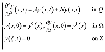(1)

and the linear part of the system (1) is

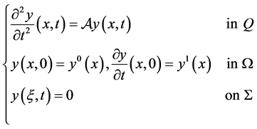(2)

where is an elliptic and second order operator and is a nonlinear operator assumed to be locally Lipschitzian, system (1) is augmented with the output function given by

(3)

where (resp. if the subregion of interest is a boundary part of the system evolution domain) is a linear operator, and depends on the number q and the nature of the considered sensors. The observation space is and assumes that

.

Let

For the system (2) is equivalent to

(4)

and the system (1) is equivalent to

(5)

augmented with the output function

(6)

with the system (4) has a unique solution see [10] - [12] that can be expressed as,

is the semigroup generated by the operator.

Let’s consider a basis of eigenfunctions of the operator, with the condition of Dirichlet which noted and eigenvalues associated are with multiplicity.

We can write for any

The system (5) has a unique solution that can be expressed as follows see [13]

(7)

then the output Equation (6) can be expressed by

Let be the observation operator defined by

which is linear and bounded with the adjoint given by

Consider the operator given by the formula

where

(resp. if the subregion of interest is a boundary part of the system evolution domain.)

is the adjoint of.

The initial condition (initial state and initial speed) and its gradient are assumed un- known. For an open subregion of, consider the restriction operators

with is the adjoint of (resp. is the adjoint of).

(resp. For, consider

and

with (resp. and) is the adjoint of (resp. and) which is the restriction operator.

The trace operator is defined by

with

and is the trace operator of order zero which is linear, continuous, and surjective. (resp.) denote the adjoint of operator (resp.).

Finally, we reconstruct the operator as follows

Definition 1

・ The system (2) together with the output (3) is said to be exactly (resp. weakly) G-observable in if

(resp.

・ The system (2) together with the output (3) is said to be exactly (resp. weakly) G-observable in if

(resp.).

Remark 1.

・ If the system (2) together with the output (3) is exactly G-observable on (resp. in) then it is weakly G-observable on.

・ For the system (2) together with the output (3) is exactly (resp. weakly) G-observable on then it is exactly (resp. weakly) G-observable on. see [9] .

Definition 2 The semilinear system (1) augmented by the output function (3) is said to be gradient observable or G-observable on (resp. in) if we can reconstruct the gradient of its state and speed on a subregion of (resp. in of).

Let the gradient of the initial condition be decomposed as follows:

(8)

where, and

Problem (*)

Given system (1) augmented by the output (3) on, is it possible to reconstruct which is the gradient of initial condition of (1) in? (resp. on.)

3. Sectorial Case

In this section, we study Problem (*) under some supplementary hypothesis on and the nonlinear operator.

With the same notations as in the previous case, we reconsider the semilinear system described by the Equ- ation (5) augmented by the output (6) where one suppose that the operator generates an analytic semigroup

in the state space E.

Let’s consider such that with a is a positive real number and

denotes the real part of spectrum of. Then for, we define the fractional power as a closed operator with domain which is a dense Banach space on E endowed with the graph norm

Let us consider then the objective is to study the Problem (*) in V endowed with the norm

(9)

we have

where c is a constant. For more details, see ( [2] [11] [14] ).

For, assume that

(10)

and the operator is well defined and satisfies the following conditions:

(11)

This hypothesis are verified by many important class of semi linear hyperbolic systems. Various examples are given and discussed in ( [14] - [16] ).

We show that there exists a set of admissible initial gradient states and admissible initial gradient speed, admissible in the sense that allows to obtain system (2) weakly G-observable.

Let’s consider

given by

where is the restriction in and is the residual part of the initial gradient condition given by (8). we assume that

(12)

then we have the following result

Proposition 1 Suppose that the system (2) is weakly G-observable on, and (10), (11) and (12) satisfied, then the following assertion hold:

・ There exists and such that for all the function has a unique

fixed point in the ball solution of the system (5).

・ There exist and such that, the mapping f is Lipschitzian where

Proof.

・ Since, then there exists such that

and we have.

Let us consider and in and we have

where

Using Holder’s inequality we take

and using (11), we have

On the other hand, we have

but we have

and

Using Holder’s inequality, we obtain

then we have

and

where.

Finally

Let’s consider,

and, , then.

It is sufficient to take and, then for all we have

・ Let and be the solution of the system (5) corresponding respectively to the initial gradient condition, we suppose that we have the same residual part (), then for we have

but we have

and we deduce that

(13)

Finally, f is Lipschitzian in.

Remark 2 The given results show that there exists a set of admissible gradient initial state. If the gradient initial state is taken in, with a bounded residual part then the system (5) has only one solution in.

Here, we show that if the measurements are in, with is suitably chosen then the gradient initial state can be obtained as a solution of a fixed point problem.

Let us consider the mapping

(14)

and assume that.

Then we have the following result.

Proposition 2 Assume that

(15)

(16)

and if the linear system (2) is weakly G-observable on Γ and (11) holds, then there exists a₂ > 0 and, such that for all , the function (14) admit a unique fixed point in which correspond to the gradient initial condition observed on. Furthermore, the function is Lipschitzian.

Proof. Let us consider and in, using ((9),(11), (13), (15) and (16)) we have

Or, then there exists such that

and we have.

Then we obtain

On the other hand, using the inequalities (11), (15) and (16), we have

Let’s consider.

In order to have, it suffices to consider.

For, we have

which gives

Then

which shows that h is Lipschitzian.

Remark 3 We can consider the regional intern problem in a subregion of (see [17] ).

4. Numerical Approach

We show the existence of a sequence of the initial gradient state and initial gradient speed which converges respectively to the regional initial gradient state and initial gradient speed to be observed on.

Proposition 3 We suppose that the hypothesis of the proposition (3.2) are verified, then for, the sequence of the initial gradient condition defined in by

(17)

converges to the regional initial gradient condition (the regional initial gradient state and the regional initial gradient speed) to be observed on. where is the residual part of the initial gradient condition.

Proof. We have,

or, then ,

Then is a Cauchy sequence on V and is convergent.

We consider and with

we have.

So

then

which show that the sequence converges to in Y on the other hand, we have

hence converges to the regional initial gradient to be observed on.

Algorithm

Let’s consider, then we have

and.

Thus, we obtain the following algorithm:

5. Simulations

In this part, we give a numerical illustrating example and the simulations are related to the choice of the subregion, the sensor location.

5.1. Internal Subregion Target

Consider the one dimensional semilinear hyperbolic system

(18)

augmented with the output function described by a pointwise sensor located in and

(19)

where is a complete set of. Let’s consider

Using the previous algorithm, we obtain the following figures.

・ Figure 1 shows that the estimate gradient state is very close to the real initial gradient state in.

・ Figure 2 shows that the estimate gradient speed is very close to the real initial gradient speed in.

5.2. Boundary Subregion Target

Consider the two dimensional system described in by

(20)

where is a complete set of.

The system (20) augmented by output function described by a pointwise sensor located in b.

(21)

with

・ , the sensor located at.

・ is the intern region.

・ is the boundary region.

・ The initials gradient conditions

to be observed on.

Using the previous algorithm, we obtain the following results:

・ Figure 3 shows that the estimate boundary gradient state is very close to the real initial boundary gradient state on.

・ Figure 4 shows that the estimate boundary gradient speed is very close to the real initial boundary gradient speed on.

6. Conclusion

The question of the regional internal and boundary gradient observability for semilinear hyperbolic systems was discussed and solved using the sectorial approach, which used sectorial properties of dynamical operators, the fixed point techniques and the properties of the linear part of the considered system. Many questions remain open, such as the case of the regional gradient observability of semilinear systems using Hilbert Uniqueness Method (HUM) and the constrained observability of semilinear hyperbolic system.

Cite this paper

Adil Khazari,Ali Boutoulout, (2016) Sectorial Approach of the Gradient Observability of the Hyperbolic Semilinear Systems Intern and Boundary Cases. Applied Mathematics,07,1326-1339. doi: 10.4236/am.2016.712117

References

- 1. Zerrik, E., Bourray, H. and Boutoulout, A. (2002) Regional Boundary Observability, Numerical Approach. International Journal of Applied Mathematics and Computer Science, 12, 143-151.
- 2. Zerrik, E., Bourray, H. and El Jai, A. (2007) Regional Observability for Semilinear Distributed Parabolic Systems. Journal of Dynamical and Control Systems, 3, 413-430.
- 3. Boutoulout, A., Bourray, H. and El Alaoui, F.Z. (2013) Boundary Gradient Observability for Semilinear Parabolic Systems: Sectorial Approach. Mathematical Sciences Letters, 2, 45-54.
http://dx.doi.org/10.12785/msl/020106 - 4. Boutoulout, A., Bourray, H. and El Alaoui, F.Z. (2012) Regional Gradient Observability for Distributed Semilinear Parabolic Systems. Journal of Dynamical and Control Systems, 18, 159-179.
http://dx.doi.org/10.1007/s10883-012-9138-3 - 5. Zerrik, E. and Bourray, H. (2003) Gradient Observability for Diffustion System. International Journal of Applied Mathematics and Computer Science, 13, 139-150.
- 6. Zerrik, E., Bourray, H. and El Jai, A. (2003) Regional Flux Reconstruction for Parabolic Systems. International Journal of Systems Science, 34, 641-650.
http://dx.doi.org/10.1080/00207720310001601028 - 7. Boutoulout, A., Bourray, H., Benhadid, S. and El Alaoui, F.Z. (2014) Regional Gradient Observability for Distributed Semilinear Parabolic Systems. International Journal of Control, 87, 1-13.
- 8. Boutoulout, A. and Khazari, A. (2013) Gradient Observability for Hyperbolic System. International Review of Automatic Control (IREACO), 6, 263-274.
- 9. Boutoulout, A., Bourray, H. and Khazari, A. (2014) Flux Observability for Hyperbolic Systems. Applied Mathematics & Information Sciences, 2, 13-24.
- 10. Pazy, A. (1990) Semigroups of Linear Operators and Applications to Partial Differential Equations. Springer-Verlag, New York.
- 11. Zeidler, E. (1990) Nonlinear Functional Analysis and Its Applications II/A Linear Applied Functional Analysis. Springer, Berlin.
- 12. Curtain, R.F. and Zwart, H. (1995) An Introduction to Infinite Dimensional Linear Systems Theory. Texts in Applied Mathematics, Springer-Verlag, New York, 138.
http://dx.doi.org/10.1007/978-1-4612-4224-6 - 13. Lions, J.L. (1988) Contr?labilité Exacte, Perturbations et Stabilisation de Systèmes Distribués. Tome 1, Masson, Paris.
- 14. Henry, D. (1981) Geometric Theory of Semilinear Parabolic Systems. Lecture Notes in Mathematics 840, Springer-Verlag Berlin Heidelberg New York.
http://dx.doi.org/10.1007/BFb0089647 - 15. Kassara, K. and El Jai, A. (1983) Algorithme pour la commande d'une classe de systmes paramtre rpartis non linaires. Revue Marocaine d’Automatique, d’Informatique et de Traitement de Signal, 1, 3-24.
- 16. Lions, J.L. and Magenes, E. (1968) Problèmes aux limites non homogènes et applications. Vols. 1 et 2, Dunod, Paris.
- 17. Khazari, A. and Boutoulout, A. (2014) Gradient Observability for Semilinear Hyperbolic Systems: Sectorial Approach. Intelligent Control and Automation, 6, 170-181.
http://dx.doi.org/10.4236/ica.2014.53019