Applied Mathematics
Vol.5 No.6(2014), Article ID:44585,6 pages DOI:10.4236/am.2014.56085
The Probability Distribution of the Elastic Properties of Pure Metals
Clint Steele
Swinburne University of Technology, Hawthorn, Australia
Email: csteele@swin.edu.au
Copyright © 2014 by author and Scientific Research Publishing Inc.
This work is licensed under the Creative Commons Attribution International License (CC BY).
http://creativecommons.org/licenses/by/4.0/


Received 12 December 2013; revised 14 January 2014; accepted 27 January 2014
ABSTRACT
While there are many published data on the average properties of elasticity for metals, there is little on the expected randomness. This is despite the known randomness of the elasticity of the grains that make up metals. It seems implicitly assumed that due to pseudo-isotropy, the average is all that is of concern. But how does one know if this is always the case? By creating a simple model of a metal, it is shown that for typical metal samples the randomness is negligible. However, as samples become smaller, it is possible to estimate the randomness based on information about the properties of grains within the metal. Further, due to the central limit theorem, which is implied by the model, a Gaussian distribution can be expected. This can be used in an evolutionary approach to generating a distribution for further probabilistic analysis of a respective system.
Keywords:Elasticity, Engineering Materials, Central Limit Theorem, Pseudo-Isotropy

1. Introduction
Probabilistic design is a sub discipline of engineering design that concerns itself with the predication and management of the effects of randomness in the values of key design variables and parameters. This discipline has been documented for some decades; now Haugen [1] is an example of the earliest texts on the topic. Much of the randomness that is experienced comes from manufacturing or material properties. For this reason, it is of value to have a realistic representation of the distribution for material properties. While Haugen argued that a Gaussian distribution can be assumed for all distributions, others, especially Siddall argued that a design engineer should use their understanding of the respective phenomena to intuitively determine a preliminary distribution [2] . This distribution would then be updated with data, as they came to hand, through an evolutionary method. It was considered by Siddall that the Bayesian approach was not flexible enough [3] . The limitation of the evolutionary approach is that it ignores the value that could be had from applying probability theory to the theory of the respective phenomena to develop an as accurate as possible preliminary distribution for the evolutionary method. This has been the focus of the author of this paper for some time. The consideration of the elastic properties of metals is one application and is the one that will be considered here.
2. Theoretical Background
2.1. The Elastic Properties of Metal Grains
Metals are constituted of grains. Within each grain, the atoms are arranged in a crystal structure. When a metal is compressed, twisted or expanded under force, the change in shape is initially accommodated by the movement of the subatomic particle (elections and the nucleus) within ach atom relative to each other.
If the force becomes great enough to cause the atoms to move relative to each other, then the deformation had become plastic. This is not within the scope of this paper and these properties require separate analysis.
The force required to cause a certain expansion is defined as the modulus of elasticity E. The modulus of elasticity for each grain is a function of the orientation of the crystals within. Thus, if the orientation of a grain is random, then the modulus of elasticity of in the direction of interest is also random. The grains within the typical sample of metal are random. This randomness can also vary depending upon treatments, which can affect the size of grains and their orientation. This random orientation of the grains within a metal sample is the source of randomness for the elastic properties in metals.
The modulus for elasticity for a metal crystal at a set orientation can be found analytically with accurate results.
2.2. Elastic Properties of Macroscopic Metals
Others have taken the models for the modulus of elasticity as a function of orientation and integrated them over all possible orientations to find the average modulus [4] . While these results have proven close to measured values, they assume pseudoisotropy (the effective isotropy that comes from have a large number random samples that average each other out), and have paid little attention to the amount and nature of random variation that can be expected.
By taking these models for a single grain and then creating a model for a larger sample, it will be possible to determine how the variability changes with the size of the sample and the average grain size. This will then provide guidance to probabilistic designers on assumptions that they should make for design variables and parameters that are essentially elastic properties of metals.
3. Analysis
3.1. Model
The first step in the analysis process is the development of a model for a metal sample. To create this model, the idealized metal sample was treated as a cube made of many other cubes as shown in Figure 1.
Each smaller cube is a grain with a random modulus of elasticity. The sample is n1 grains wide n2 grains high and n3 grains long.
In this case the modulus of elasticity in the horizontal direction is to be considered. First consider the left most plane consisting of n1 by n3 grains. If the grains are fixed to each other, then each grain will experience the same change in length X’ after being subjected to the force F.
According to Hook’s Law, the relationship between force and elastic deformation is
 (1)
(1)
where:
• s is the stress F/A;
• e is the engineering strain X/L;
• A is the area over which the force is acting.
If both X’ and L’ are the same for each grain in the left most plane, then it is only the modulus E’ and stress s’ that will change from grain to grain. The engineering strain for each grain throughout the plane considered is equal and given the symbol ep.
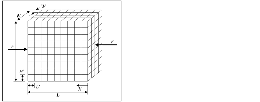
Figure 1. Simplified metal structure.
Additionally, the total force that is experienced by the grains in the first plane will be the sum of the force from each grain F’ and be equal to the total force applied F. This is expressed mathematically in Equation (2).
 (2)
(2)
To take advantage of Hook’s law the expression must be in terms of stress and strain. Thus, both sides of Equation (2) becomes
 (3)
(3)
Noting that A/A’ is equal to n1 n2, Equation (3) can be modified as
 (4)
(4)
The stress s can now be replaced with modulus elasticity E and strain e by using Hook’s law
 (5)
(5)
Note the use of Ep for the modulus of elasticity for the plane in question and the strain for the plane ep, which cancels out to give
 (6)
(6)
With an expression for Ep, the next required step is to find a relationship between Ep and E.
Consider n2 planes stacked next to each other to complete the metal sample. The area of each plane is the same and the force acting on each plane is the same. Therefore, the stress each plane is subjected to resulting from the force F is the same. The length L of the sample is equal to the summation of the length of the planes L’. Also, the total elastic deformation of the sample X is equal to the summation of the elastic deformation of the planes X’. These can be expressed as
 (7)
(7)
and
 (8)
(8)
respectively.
The strain for the sample e when subjected to the force F then becomes
 (9)
(9)
The deflection X’ can be replaced with the strain for the respective plane ep multiplied by the length L’
 (10)
(10)
In this simplified model L’ is a constant and can be removed from the summations to cancel out in Equation (10), leaving
 (11)
(11)
Returning to Hook’s law, the strain of the plane in Equation (11) can be replaced with the modulus of elasticity for that plane ep and the stress that all planes are equally subject to s. This results in
 (12)
(12)
The stress s, being constant, can be brought to the left of Equation (12). This will then bring about the overall strain e being divided by the overall stress s, which is equal to the reciprocal of modulus of elasticity for the sample being analysed:
 (13)
(13)
Note that the number of grains along the length n3 has been brought out of the summation in Equation (13). Equation (13) can now be reciprocated to produce an expression for the modulus of elasticity E:
 (14)
(14)
Together, Equation (6) and Equation (14) provide a model for the modulus of elasticity for a sample metal as a function of the random modulus of elasticity for each grain.
By applying the moment method to Equation (6) the expected value Epd[ ] for Ep can be had,
 (15)
(15)
As can the standard deviation Std[ ] for Ep,
 (16)
(16)
Applying the moment method to Equation (14) the first order approximation for the expected value of E is found to be
 (17)
(17)
Thus the average value of elasticity for a metal sample is that of a single grain’s over its possible orientations. This has been done by others and good results (when compared to measurement were found). However, it is the standard deviation and the shape of the distribution that is of interest to the probabilistic designer.
The moment method can be used again to find the first order approximation for the standard deviation of the modulus of elasticity as a function of the standard deviation of the modulus of elasticity of a plane. The outcome is
 (18)
(18)
By substituting Equation (16) into Equation (18) a final expression can be had for the standard deviation of the modulus of elasticity for a large sample, made of a number N of grains. This expression is
 (19)
(19)
3.2. Model Application
To evaluate the application of this probabilistic model and to assess the insights it can provide, the case of tin will be considered. On a granular level the maximum modulus of elasticity for tin is 84.4 GPa and the minimum is 24.4 GPa. With only the maximum and minimum values available, a uniform distribution is the least biased assumption. Thus the mean and standard deviation of E’ in this case are 44 GPa and 17 GPa respectively. The observed average modulus elasticity for tin is 45.6 GPa [4] , but the author was unable to find published values for the standard deviation.
With the above information it is possible to plot the standard deviation as a function of the number of grains for tin. However, it is impractical to specify a metal sample by the number of grains within. Instead, the basic dimension of the sample D and the average grain size d are easier to consider and specify. The relationship between N, D and d is
 (20)
(20)
By inserting Equation (20) into Equation (19), an expression for the standard deviation of the modulus of elasticity in terms of the grain size and sample size is at hand:
 (21)
(21)
Using the values for tin above it is possible to plot Equation (21) as shown in Figure 2.
3.3. Model Implications
Because Equation (6) is a series of summations, via the central limit theorem the distribution for Ep can be assumed to be close to Gaussian. Equation (14) also has a series of additions. However, there is also a reciprocation. The reciprocal function is much like a linear function when the value of the input is large. Further, if the mean of the input is large in comparison to the standard deviation, then the effects of any minor non-linearity is minor, and the output distribution is much the same type as the input. Thus, if the standard deviation of Ep is small relative to the mean, then the distribution of the modulus of elasticity is likely very close to a Gaussian distribution.
Typically, grains are less than a millimetre in size and can be as small as one one-hundredth of a millimetre. Typical engineered parts are from tens of millimetres to metres. Thus the ratio of D to d is around 100 or more. From inspection of Figure 2, this corresponds to a negligible standard deviation of the modulus of elasticity. This means further that the standard deviation is small compared to the mean, and that the distribution, while very narrow, is well approximated by a Gaussian distribution.
Because the other elastic properties of metals have the same sources of randomness [4] , the conclusions about the modulus of elasticity are valid for other properties such as the modulus of rigidity and Poisson’s ratio.
4. Conclusions
Through the application of a simple model it can be seen that the modulus of elasticity for a typical engineering metal sample will have negligible randomness. This is due to the large number of grains in a typical sample, the random orientation of the grains and the central limit theorem. This negligible value is likely the reason why there are little published data on the randomness of elastic properties of metals.
However, as a sample becomes smaller, which is becoming more likely with advances in nano technology, it is likely that this assumption is no longer valid. In such cases though, an engineer can use the derived models (and published data about metal grains [4] ) to provide an estimation of the expected randomness. It can also
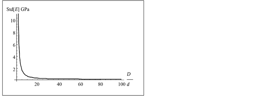
Figure 2. Grain size and standard deviation for tin.
likely still be assumed that the distribution will be Gaussian, as per the central limit theorem. The engineer can then use this distribution for further probabilistic analysis of the respective system being designed.
References
- Haugen, E.B. (1968) Probabilistic Approaches to Design. John Wiley and Sons Inc, USA.
- Siddall, J. (1984) A New Approach to Probability in Engineering Design and Optimization. Journal of Mechanisms, Transmissions, and Automation in Design, 106, 5-10. http://dx.doi.org/10.1115/1.3258562
- Siddall, J. (1986) Probabilistic Modeling in Design. Journal of Mechanisms, Transmissions, and Automation in Design, 108, 330-335. http://dx.doi.org/10.1115/1.3258735
- Schmid, E. and Boas, W. (1950) Plasticity of Crystals. F.A. Hughes, London.