ABSTRACT

Received September 21, 2013; revised October 21, 2013; accepted October 28, 2013

This work deals with the relationship between the Bayesian and the maximum likelihood estimators in case of dependent observations. In case of Markov chains, we show that the Bayesian estimator of the transition proba- bilities is a linear function of the maximum likelihood estimator (MLE).

Keywords:

Bayes Estimator; Maximum Likelihood Estimator; Markov Chain; Transition Probabilities; Jeffreys’ Prior; Multivariate Beta Prior; MCMC

1. Introduction

Let be the random variable with Bernoulli distribution with parameter. It’s known that the Bayesian solution, under quadratic loss and a beta distribution as prior for, is given by

(1.1)

with and. If is a sample from, the Bayesian estimate becomes

(1.2)

with and.

Moreover, is the MLE which coincides with the empirical estimate.

Formulas (1.1) and (1.2) are still true with distribution of in the exponential family [1].

Let’s now move to the dependent case and show that (1.2) is still true for the Markov chains.

Let be the first observations of an homogeneous Markov chain with a finite state space and let be the matrix of transition probabilities. The likelihood is

(1.3)

where.

Let 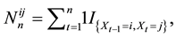which gives the number of one step transition from to until time,

then (1.3) becomes

(1.4)

The parameter is to be estimated, and we assume that the distribution of

is known, that is with is known. Then, the MLE of is given by

(1.5)

which coincides with the empirical estimate.

The Bayesian estimator under the quadratic error loss, is given by

(1.6)

where is the posterior distribution. Two conjugate prior distributions are viewed. The multivariate beta distribution [2] and the Jeffreys’ distribution [3].

This work is organized as follows: In the second Section, we develop the Bayesian estimation for different priors. In Section 3, the cases of 2 and 3 states Markov chain are discussed. A numerical study is given in Section 4.

2. The Bayesian Framework

In this section, we introduce two conjugate prior distributions for of a multistate Markov chain. The first kind of these priors is the product of the multivariate beta which doesn’t take account of a possible correlation between the rows of transition probability matrix. The second kind is the Jeffreys’ prior [3] which incorporates a certain type of dependence between the components of the parameter.

2.1. Multivariate Beta Priors

Given the characteristics of the transition probabilities, the natural choice of prior distributions is the multivariate beta distribution [2]. Thus, let the prior distribution for the elements of the row of the matrix be the multivariate beta, that is,

(1.7)

where denotes the gamma function.

There are rows in the transition matrix and thus there are such prior’s in (1.7). If the rows of are assumed independent then the joint prior probability density function for all is

(1.8)

Making use of the likelihood given by (1.4) and the prior in (1.8), the joint posterior is

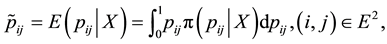
The Bayesian estimator of corresponding to the multivariate beta is then given by

(1.9)

Let us remark that the Bayesian estimator can be written as

with and. The above relation seems to

be compared to (1.2), but here, the coefficients and depend also on the sufficient statistics.

2.2. The Jeffreys’ Prior

Assoudou and Essebbar [3] have studied the Bayesian estimation for the multistate Markov chains, under the Jeffreys’ prior distribution. As shown, this prior has many advantages: it permits a certain type of dependence between the various transition probabilities. Moreover it’s a conjugate prior for given by (1.4). The absence of extra parameter in this prior is of great interest, because we don’t need to do more extra estimation.

The Jeffreys’ prior and the correspondent posterior distributions [3] are respectively given by

where is the stationary probability and is the probability that the initial state is.

One can deduce the Jeffreys’ prior and posterior distributions for the two-states Markov chain,

(1.10)

(1.11)

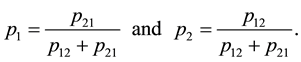
where and is the stationary probability given by

For the three-states Markov chain with parameter, the prior and the posterior Jeffreys’ distributions are respectively

(1.12)

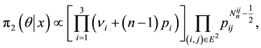(1.13)

where the stationary probability is given by

3. The Bayesian Solution

For either posterior distributions (1.11) or (1.13), the integral given by (1.6) is difficult to calculate, so we propose an approximation of it by mean of an algorithm, namely the Independent Metropolis-Hasting algorithm (IMH) [4].

The fundamental idea behind these algorithms is to construct an homogeneous and ergodic Markov chain with stationary measure.

For “large enough”, is roughly distributed from and the sample can be

used to derive the posterior means. For instance, the Ergodic Theorem [4] justifies the approximation of the integral (1.6) by the empirical average

in the way that is converging to the integral (1.6) for almost every realization of the chain under minimal conditions.

For next, we will give the description of this algorithm in the cases of two-states and three-states.

1) Case of the two-states Markov chain

Given

・ Step1. Generate

・ Step2. Take

where

・

・ is the posterior density given by (1.11).

2) Case of the three-states Markov chain

Given

・ Step1. Generate such as:

1) Generate until

2) Generate until

3) Generate until

・ Step2. Take

where

・ is the posterior density given by (1.13).

4. Numerical Study

In order to characterize the relationship between the Bayesian estimator and the MLE, it’s indispensable to perform simulation studies. The first part of the analysis is devoted to Bayesian model founded on the multivariate beta prior given by (1.8) while the second deals with the Bayesian model using the Jeffreys’ prior given by theorem 1. We discuss through this analysis the cases of Markov chain with two and three states.

In both experiments, a pascal program is written to run the transition probabilities. The Bayesian estimator corresponding to Jeffreys’ prior is obtained from a single chain including iterations of IMH algorithm (Section 3).

4.1. Experiment (a)

In Section 2.1, we have shown that, under the multivariate beta prior, the analytical Bayesian solution doesn’t express clearly a certain linearity of the MLE. In this experiment, we demonstrate by simulation that the Bayesian estimator given by (1.9) is a linear function of the MLE given by (1.5).

4.1.1. Case of the Two-States Markov Chain

The data set is composed of 100 independent two-states Markov chains with 20 observations. To generate this data set, transition probabilities for each chain are drawn from the beta prior given by (1.8) with and parameters. The first state , in each chain, is assumed to be equal to 1. The remaining observations given each chain, are then simulated in succession according to the appropriate transition probabilities. The Bayesian estimator for each chain, is computed from (1.9).

Figure 1(a) (resp. Figure 2(a)) shows the plot of (resp.) versus (resp.). These figures prove that the Bayesian estimator is quite a linear function of the MLE.

4.1.2. Case of the Three-States Markov Chain

In this experiment we generate 100 independent Markov chains each with three states and 60 observations. By using the IMH algorithm, the transition probabilities are simulated from the multivariate beta given by (1.8) with and parameters. As previously, the Bayesian estimator is calculated from (1.9). The plots of versus are given by the next figures (Figure 3(a) until Figure 8(a)). It’s true that the linearity of the Bayesian estimates is still verified, but we remark that the plot is not quite a line as soon as the number of states grows.

4.2. Experiment (b)

Now let us consider the Bayesian model based on the Jeffreys’ prior such that described in Section 2.2.

4.2.1. Case of the Two-States Markov Chain

In this experiment, we simulate 100 independent two-states Markov chains with, obviously the chains may be of differing lengths. The IMH algorithm is first used to generate the transition probabilities from the Jeffreys’ prior given by (1.10). We assume, without loss of generality, that the first state , in each chain, is equal to 1 (). The remaining observations, in each chain, are then simulated in succession with the appropriate transition probabilities. To obtain the Bayesian estimator of the transition probabilities given each chain, we apply the IMH algorithm to the posterior distribution given by (1.11). The MLE is calculated from (1.5).

Figure 1(b) (resp. Figure 2(b)) displays the plot of (resp.) versus (resp.). From these figures it follows clearly that the Bayesian estimator is a linear function of the MLE.

4.2.2. Case of the Three-States Markov Chain

The same experiment is repeated once more, but now the transition probabilities are drawn from the Jeffreys’ prior given by (1.12) in order to gererate 100 independent three-states Markov chains with. The Bayesian estimator is approximited by mean of IMH algorithm applied to the posterior distribution given by (1.13).

The next figures (Figure 3(b) until Figure 8(b)) show the plots of versus. The same results as in Section 4.1.2 are obtained about the relationship between the Bayesian estimator and the MLE.

5. Conclusion

The objective of this work is to study the relationship between the Bayesian estimator and the MLE in a dependent case such as a Markov chain. A numerical study by simulation is carried out to describe the nature of this relationship. Under the multivariate beta and the Jeffreys’ priors we have shown that the Bayesian solution is still a linear function of the MLE. This linearity is now verified by simulation for these two models, others

simulation will be developed for different Bayesian models. The next step will be to proof analytically this property.

References

- P. Diaconis and D. Ylvisaker, “Conjugate Priors for Exponential Families,” The Annals of Statistics, Vol. 7, No. 2, 1979, pp. 269-281.
- T. C. Lee, G. G. Judge and A. Zellner, “Maximum Likelihood and Bayesian Estimation of Transition Probabilities,” JASA, Vol. 63, No. 324, 1968, pp. 1162-1179.
- S. Assoudou and B. Essebbar, “A Bayesian Model for Markov Chains via Jeffreys’ Prior,” Department of Mathematics and Computer Sciences, Faculté des Sciences of Rabat, Morocco, 2001.
- C. Robert, “Méthode de Monte Carlo par Chanes de Markov,” Economica, Paris, 1996.