Applied Mathematics
Vol.4 No.7(2013), Article ID:34109,14 pages DOI:10.4236/am.2013.47138
Eigenanalysis of Electromagnetic Structures Based on the Finite Element Method
Department of Electrical and Computer Engineering, Microwaves Lab., Democritus University of Thrace, Xanthi, Greece
Email: gkyriac@ee.duth.gr
Copyright © 2013 C. L. Zekios et al. This is an open access article distributed under the Creative Commons Attribution License, which permits unrestricted use, distribution, and reproduction in any medium, provided the original work is properly cited.
Received February 28, 2013; revised March 29, 2013; accepted April 8, 2013
Keywords: Eigenanalysis; Finite Element Method; Open Radiating Structures; Electrically Large Cavities
ABSTRACT
This article presents a review of our research effort on the eigenanalysis of open radiating waveguides and closed resonating structures. A two dimensional (2-D) hybrid Finite Element method in conjunction with a cylindrical harmonics expansion is established to formulate the open waveguide generalized eigenvalue problem. The key element of this approach refers to the adoption of a vector Dirichlet-to-Neumann map to rigorously enforce the continuity of the two field expansions along a truncation surface. The resulting algorithm was able to evaluate both surface and leaky eigenmodes. The eigenanalysis of three dimensional (3-D) structures involves vast research challenges, especially when they are electrically large and open-radiating. The effort herein is focused on the electrically large case including the losses due to the finite conductivity of metallic walls and objects as well as the loading material losses. The former is introduced through impedance or Leontovich boundary condition, resulting to a non-linear-polynomial generalized eigenvalue problem. A straightforward linearization solution is adopted along with a more efficient alternative technique which mimics analytical approaches. For this one the linear eigenproblem formulated assuming metals as perfect electric conductors is initially solved and their finite conductivity is accounted through impedance boundary conditions enforced locally on the resulting eigenvectors. Finally, some numerical results are presented to verify the performance of these methodologies along with a discussion on their possibilities for extension to open 3D structures as well as to characteristic modes eigenanalysis.
1. Introduction
The interest in the analysis and design of waveguiding and cavity structures is always of high priority in the microwave community. The tense of this era for the utilization of even more complex and smart microwave devices and the increase of the required frequency band, demands the genesis of “smart” techniques. One idea uprise in our laboratory is the development of the eigenanalysis for the evaluation and exploitation of the modal characteristics of the studying structure. In this manner the physical properties of each structure are revealed and thus the eigenanalysis provides the guidelines for its analysis.
Valuable analytical eigen-solutions of canonical cross section closed waveguides are well established since the early days of microwaves. Arbitrary cross-section waveguides, partially or inhomogeneously loaded with either isotropic or anisotropic materials can also be studied with the aid of numerical techniques and particular the Finite Element Method (FEM), e.g. [1].
Addressing the first steps of this effort a hybrid Finite Element in conjunction with a cylindrical harmonics expansion is established for the analysis of open waveguides. The unbounded solution domain is truncated by enclosing the FEM subdomain (inhomogeneous waveguide) within a circular contour, where the field outside of that is expanded into cylindrical harmonics. The transparency of the fictitious circular contour truncating the finite element mesh is ensured by enforcing the field continuity conditions according to a vector Dirichlet-toNeumann mapping (DtN) [1]. The resulting generalized eigenproblem is extremely nonlinear due to the presence of the unknown eigenvalue (complex propagation constant) within the argument of the cylindrical Bessel functions. The approximation corresponding to the physical condition of wave cut-off in the axial direction (almost transverse propagation), yields an approximate linearized eigenproblem. Even though this seems a rough approximation is proved to be quite accurate for the major part of the eigenspectrum covering both surface and leaky modes. For the remaining part of the spectrum, the nonlinear eigenproblem is solved using an iterative RegulaFalsi technique, in conjunction with Arnoldi algorithm, by exploiting the approximate linear eigenproblem results as starting values.
For the extension to three dimensional open radiating cavities (e.g. cavity backed antennas) the finite element method can be bind together with the corresponding spherical harmonics expansions of the free space. The continuity of the field will be now enforced on a transparent fictitious spherical surface, strictly following a Dirichlet-to-Neumann mapping formalism. Once again the resulting generalized eigenvalue problem is non-linear since the unknown eigenvalue (complex resonant frequency) occurs within the arguments of the spherical Bessel functions. Different linear approximations are currently considered in order to acquire a good starting solution to be exploited in the solution of the non-linear eigenproblem. However, the extreme nonlinear nature of this problem is an open challenge which we try to overcome with newly developed techniques.
Aiming at the eigenanalysis of electrically large three dimensional structures the effort is currently restricted to closed geometries, like the reverberation chambers or focused microwave cavities. For this purpose the initial Finite Element eigenanalysis formulation is extended accordingly [2]. For the first approach a brute force technique have been applied where the whole structure is discretized and solved respectively, while in parallel an eigenvalue domain decomposition technique is under development. However, working toward an efficient and realistic modeling of these electrically large structures, numerous challenging problems are encountered. In particular when finite conductivity losses are included through an impedance or Leontovich boundary condition, the eigenproblem becomes nonlinear. A methodology of evaluating losses effects and particularly the quality factors within practical accuracies by just solving the linear eigenproblem resulting from perfect electric boundary conditions is devised by our group [3]. In particular, the eigenproblem is formulated and solved assuming cavity walls and the metallic object surface as perfect electric conductors. The resulting linear eigenproblem is solved to yield modal eigenfunctions which for the Neumann data (normal electric and tangential magnetic field components) are of practically acceptable accuracy all over the solution domain including the neighborhood of the metallic surfaces. These are in turn exploited for the evaluation of the Dirichlet boundary data (tangential electric and normal magnetic field) through the Leontovich boundary condition. Hence, finite conductivity losses are incorporated into the modal eigenfunction through this post-processing.
This article concludes with a discussion on some thoughts on how to handle the challenges brought up by the eigenanalysis of open three dimensional structures, especially the non-linearity. Additionally, some proposals are entrusted for future extensions to the formulation and solution of characteristic modes for open structures as well as for the periodical ones.
2. Hybrid Finite Element Method for Open Waveguides
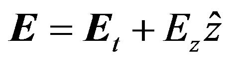
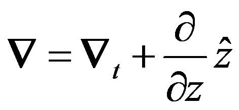
The geometry of an arbitrary cross section, inhomogeneously loaded open waveguiding structures enclosed within a circular separation contour-C is shown in Figure 1. Time harmonic fields as ejωt and propagation along the z-axis as e−jβz are assumed. The field vectors as well as the nabla operator are discriminated into transverse (t-subscript) and longitudinal components (z-components) as:
 (1)
(1)
 (2)
(2)
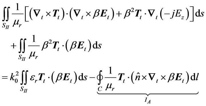
Inside the contour-C (region II) the vector wave equation for the electric field is considered and the standard Galerkin procedure is applied to yield a weak formulation of the form [1]:
Bounded Region II:
 (3)
(3)
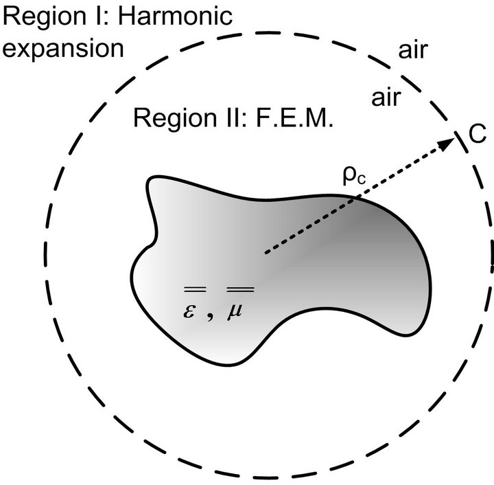
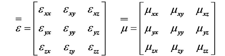
Figure 1. General open radiating waveguide geometry.
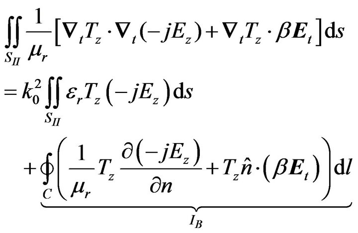 (4)
(4)
where 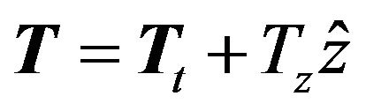 is the vector weighting function and SII the area of the bounded region-II. The contour integrals IA and IB along the fictitious contour-C, constitute the means for coupling the FEM-field inside-C to the field expansion outside-C. This coupling strictly follows the vector Dirichlet-to-Neumann (DtN) mapping, which ensures the transparency of this fictitious contour, e.g. Givoli [4,5].
The field in the unbounded region-I is expressed as a superposition of TEz and TMz modes, which according to classical Jackson textbook [6] constitute a complete set of vector solution to Maxwell equations. The longitudinal components in unbounded Region I read:
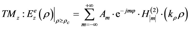 (5)
(5)
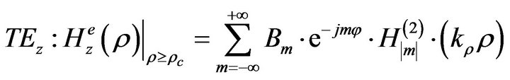 (6)
(6)
where 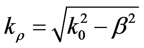 is the radial wavenumber and
 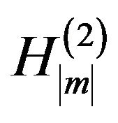 the Hankel functions of the second kind. Since, β is the unknown complex eigenvalue its presence in the argument of the Hankel functions through kρ causes the problem non-linearity.
Following a standard waveguide analysis, e.g. Pozar [7], the transverse field components are expressed in terms of their axial counterparts (5), (6) by expanding Maxwell curl equations in Cartesian coordinates [1].
Dirichlet to Neumann mapping: For the coupling of the field expression inside and outside-C the vector DtN principles are in turn applied. Its first step requires that “the solution in the unbounded region-I to be constructed from Dirichlet data on the separation contour-C”. Since, the electric field wave equation is solved using FEM in the interior of C, then the Dirichlet data are comprised of the tangential field components ,
, . Hence, the related field continuity conditions read:
 (7)
(7)
 (8)
(8)
Exploiting the orthogonality properties of the azimuthal eigenfunctions e−jmφ the unknown coefficients Am, Bm of the expansion are evaluated [1] through Equations (7) and (8). Namely, this step has indeed established the solution in the unbounded domain (region I). The DtN second step reads “establish a Dirichlet-to-Neumann map on the separation contour-C by differentiating the solution in the unbounded domain with respect to the transverse-radial ρ-coordinate and enforce their continuity across-C”. Since, the Dirichlet data are comprised of the electric field, the differentiation with respect to ρ-coordinate is given by the Maxwell Curl equation  which yields the magnetic field tangential components all over region I
  and
and . The
. The ,
,  values on the C-contour comprise the Neumann data. Their availability enables the evaluation of the coupling integrals IA, IB through the enforcement of the tangential magnetic field continuity.
 (9)
(9)
 (10)
(10)
The coupling integrals IA, IB of the weak formulation (3) and (4) are then rewritten by means of Maxwell Curl equations in cylindrical coordinates as:
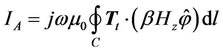 (11)
(11)
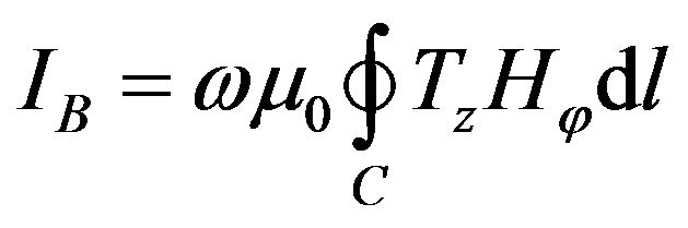 (12)
(12)
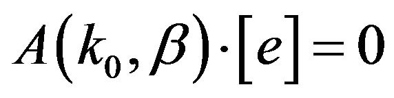
The substitution of (9), (10) into (11), (12) and through that in (3) and (4) concludes to the final “equivalent closed hybrid FEM formulation”. This is in turn discretized over the whole region-II included within the contour-C using the interpolation functions for hybrid edge/ node triangular elements (line elements for C) according to [8]. The resulting expressions are then separated into a group of terms involving the unknown eigenvalue  and terms independent of that to yield a non-linear generalized eigenvalue problem [1]:
 (13)
(13)
The eigenvalues of (13) are the complex propagation constants of the waveguiding structure.
Discussion on Uniqueness: It’s worth noting that the DtN procedure described above contradicts the electromagnetic uniqueness theorem which states that the enforcement of either tangential electric field or tangential magnetic field continuity on the contour-C yields a unique solution. In contrary, DtN presumes the enforcement of both electric and magnetic field continuity. However, the DtN provisions were indirectly well established by Prof. Harrington in 1989 [9], who states that enforcement of both conditions is absolutely necessary in order to avoid matrix singularities at the frequencies of internal resonances. At this point one may recall that the propagation constants are the solutions of some kind of a characteristic equation which is identical to the transverse resonance condition. Hence, this is indeed a condition of internal resonance and both tangential electric and tangential magnetic field continuity conditions must be enforced. Additional support to the above statement is provided by the algebraic manipulations necessary to obtain analytical eigensolutions for canonical open waveguides. It is well understood for example that in order to extract the modal characteristic equation for a dielectric slab or cylindrical dielectric rod both tangential electric and tangential magnetic field continuity must be enforced across the dielectric-air interface.
Non linearity and equivalent linear eigenproblem: Equation (13) represents a non-linear generalized eigenproblem, since the unknown eigenvalue  occurs in multiple terms but also within the argument
 of the Hankel functions in (5) and (6).
Hence, for the solution of (13) a good initial guess is inevitable, which can be in turn improved employing a Matrix Regula Falsi method [10]. The necessary starting solutions are obtained by formulating and solving an approximate linear eigenvalue problem. The latter is established by approximating the argument of the Hankel functions involved in the field expansion in the unbounded region-I, as:
 (14)
(14)
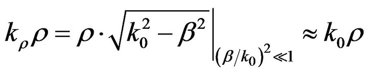
This approximation yields a linear eigenvalue problem which is solved employing the Arnoldi algorithm [11] which efficiently handles the involved sparse matrices. Although, this approximation was expected to work well around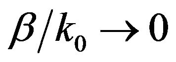 , however it was proved to perform quite well for
  up to 0.8 [1]. This makes it a valuable tool for the study of both Surface and Leaky waveguide structures since a single solution of the linear eigenvalue problem yields the entire spectrum of the complex propagation constants. It will also be shown in the numerical results section that the results of the linear approximation require improvement using the non-linear eigenvalue formulation only around the frequency ranges of high leakage (attenuation) constants. The method is validated against previously published numerical and experimental results and for open waveguiding structures first studied by our group.
Future improvements: The major limitation of the above method is related to the high computational cost of the “global radiation condition” resulting from the enforcement of the artificial truncation Contour-C transparency through the DtN approach. One part of this is unavoidable which is related to the creation of a dense area within the otherwise sparse system matrix and this is inherent to global transparency conditions. This is actually the cost to be paid for the gain of accurate transparent condition. However, most of the additional computations devoted to the calculation of the integrals along the artificial contour-C, involve far away located linear segments which add negligibly to the total numerical sum. Hence these will not compromise the numerical accuracy when omitted. The question is how to devise a methodology predicting the negligibly contributing terms without calculating them. One idea is to restrict the integral on some certain neighbourhood around each linear segment. The experience provided by similar approaches utilized within Fast Multipole methodologies e.g. [12], (which face similar drawbacks) will be exploited in our case. It must be noted that the computational cost in the 2D case is still affordable, but for the 3D open eigenproblems these integral truncations are inevitable. Finally, note that a similar compromise is made when truncating the theoretically infinite number of modes in the unbounded domain field expansion. In any case, terms contributing to the integral of the same order as the error tolerance can be neglected without any actual accuracy compromise.
Another ambitious task refers to the extension to periodic waveguiding structures, by incorporating a Floquet field expansion within FEM formulation and/or enforcing periodic boundary conditions. This approach may enable the rigorous analysis of numerous periodically located transmission lines (e.g. strips and dielectric rods) supporting important electromagnetic band gap phenomena.
3. Evaluation of Complex Resonant Wavenumber of Electrically Large Cavities
Aiming at the eigenanalysis of electrically large structures a reverberation chamber is considered as an indicative example. The most important aim of this work is to accurately calculate the imaginary part of the resonant wavenumber, which corresponds to the quality factor of each resonant eigenmode. For this purpose two different approaches are developed. First a straightforward approach is adopted, where the finite walls conductivity is taken into account by incorporating into the FEM formulation the Leontovich Impedance boundary condition. This yields a polynomial eigenvalue problem which although it can be easily linearized, the rank of the eigenproblem is increased demanding augmented computer resources which are proved to be beyond those of an ordinary desktop computer. To overcome this difficulty an alternative novel technique is established. Within this a linear eigenvalue problem is formulated and solved assuming all metallic structures as perfect electric conductors (PEC). In turn the resulting eigenfunctions (modal field distributions) are utilized for the calculation of the metals finite conductivity losses through a post processing enforcement of the Leontovich boundary condition.
3.1. 3D Eigenproblem Formulation
The simplified model of a reverberation chamber shown in Figure 2 is considered at the first steps. It is a closed metallic cavity containing the antenna the Equipment Under Test (EUT) and the metallic mode stirrer. All the metallic cavity’s walls, the mode stirrer’s the antenna’s and the EUT’s walls are assumed to have finite conductivity. The whole structure including the objects’ perturbing the cavity is simulated using FEM, employing edge elements.
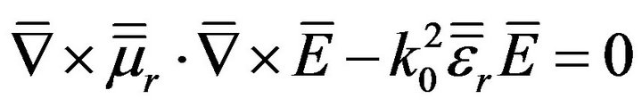
Aiming at a general formulation, an arbitrarily shaped three dimensional computational domain V inhomogeneously loaded with in general anisotropic material described with the aid of tensor permittivity  and permeability
 , is assumed. Its electromagnetic behavior can be characterized by the electric field vector wave equation which in the absence of any exciting source, reads:
 (14)
(14)
Applying a standard Galerkin procedure the following weak formulation can be derived, e.g. [13]:
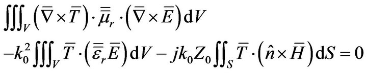 (15)
(15)
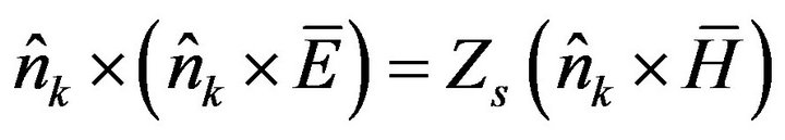
The surface integral is defined over the surface enclosing the solution domain (cavity walls) as well as on the surface of any object existing within the cavity. It is through this integral that general impedance boundary conditions are enforced within the FEM formalism. Specifically this integral serves to introduce conductor losses, according to the Leontovich boundary condition:
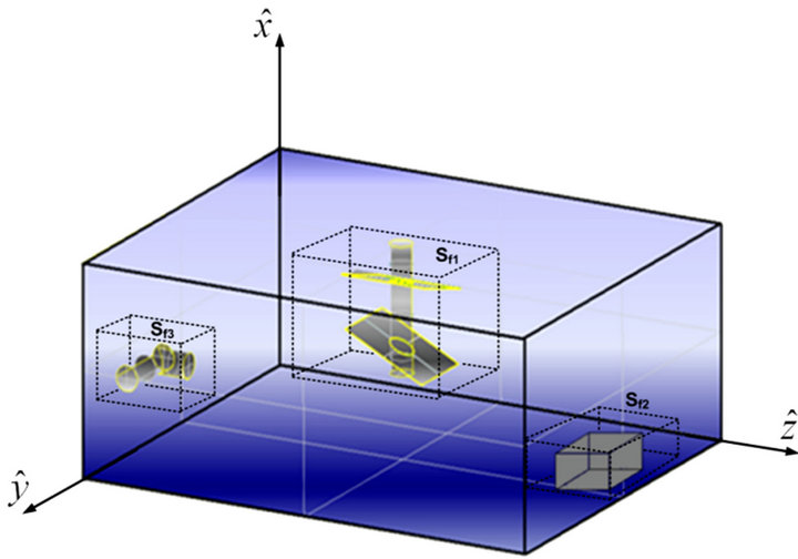
Figure 2. A simplified reverberation chamber model comprised of an inhomogeneously loaded cavity with the antenna the EUT (equipment under test) and the metallic mode stirrer.
 (16)
(16)
 is the inward unit normal vector and Zs is the surface impedance of the form [13]:
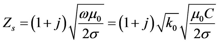 (17)
(17)
where the metallic walls are considered non-magnetic with μ = μ0, σ their conductivity and C the speed of light.
Substituting condition (16) in the formulation and taking into consideration the fact that the inward unit vector is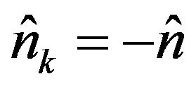 , Equation (15) becomes:
 (18)
(18)
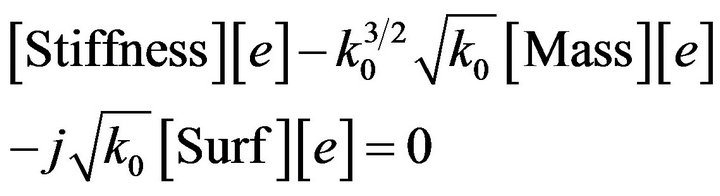
The resulting system of equations after the discretization of (18) is in turn formulated into a nonlinear generalized eigenvalue problem, by separating the terms involving the free space wavenumber k0 (or the circular frequency ω, as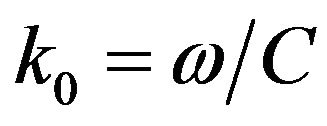 ). The final matrix form can be formulated as a nonlinear eigenvalue problem for the unknown resonant wavenumber (eigenvalues k0) as:
 (19)
(19)
where [e] is a vector comprised of the electric field values at the middle of element’s edges. The polynomial eigenvalue problem obtained above can be solved using a symmetric or companion linearization described in Subsection 3.4.
3.2. Perturbation Technique
When a magnetic sample or a dielectric material as well as any other object is placed in a large cavity, its resonance frequencies are altered. The amount of resonant frequency shift depends on the properties of the material and is proportional to the imposed energy variation. For a large cavity and a relatively small inserted object the phenomenon can be described within a practical accuracy by the “Perturbation principle”, which according to Harrington [14] reads:
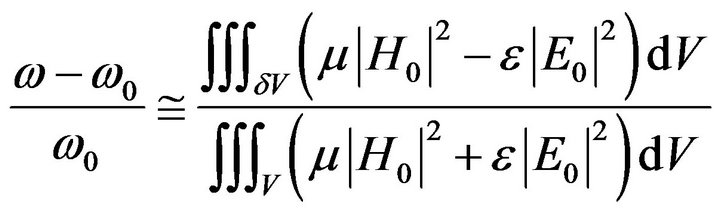 (20)
(20)
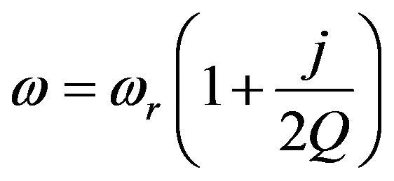
where 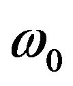 is the initial circular resonant frequency of the unperturbed cavity, ω is the resonant circular frequency after the perturbation, δV is the inserted object volume and V is the volume of the whole cavity-structure. Hence, (20) indicates that the variation in resonant frequency depends on the object’s position as well. When the dielectric and conductor losses of the cavity and the introduced objects are considered, then both ω and ω0 become complex, as:
 (21)
(21)
where  is the real resonant frequency and Q is the quality factor.
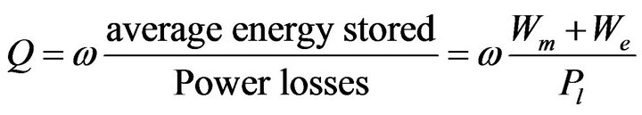
3.3. PEC Eigenanalysis for the Quality Factor Evaluation
In general the quality factor is calculated from the field distribution inside the cavity using the equation:
 (22)
(22)
where Wm and We are the magnetic and electric stored energy respectively. The power dissipated in any good conductor is classically known as the Joule losses (proportional to ), hence the same principle applies for the finite conductivity cavity walls as well as for any metallic object inserted in the cavity. The material losses (objects in the cavity) are accounted through the imaginary parts of the permittivity
  and the permeability
 . The totally dissipated power reads:
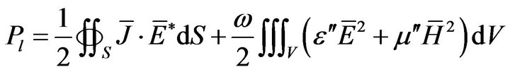 (23)
(23)
Equation (23) is general and can be used whenever the electric and magnetic field within the cavity are available either from an analytical or a numerical solution. However, even for an empty cavity the exact boundary conditions on a finite conductivity wall are complicated, depend on frequency (dispersion) and known as impedance conditions. A good approximation usually adopted is that of Leontovich given in Equation (16). But, the main difficulty with (16) is that it introduces a coupling across the walls between the electric and the magnetic field. Hence, even for an empty or homogeneously filled cavity the electric and the magnetic field wave equations cannot be exactly solved separately. Correspondingly, there are not pure TE and TM modes any more but those become hybrid. An exact analytical solution is in turn very difficult and it requires sophisticated techniques or a numerical approach. However, this coupling effect is proved to be a local phenomenon restricted around the finite conductivity conductors, while away from them the TE and TM mode eigenfunctions are retained. A very rough approximation calculates the finite conductivity losses considering this local phenomenon as a plane wave incident on the metallic walls. This yields a simplified expression often used in practice [15], which does not discriminate between different modes. A classical approach usually used for the eigenanalysis of canonically shaped cavities provides each mode quality factor with a sufficient accuracy. This is based on the modal field distributions evaluated analytically considering PEC walls (ignoring metallic losses). This approach was recently proved by our group to perform impressively well for arbitrary shaped cavities by utilizing numerical eigenfunctions which are calculated assuming PEC metallic surfaces [3]. Besides these approximations, including the conductor losses within the formulation as in (18) requires a numerical solution of the resulting non-linear eigenvalue problem, but it yields the true eigenfunctions and the related accurate quality factors.
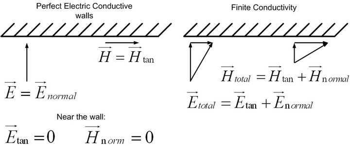
PEC versus Exact Non-Linear Eigenproblems The finite wall conductivity can be considered as a perturbation of the corresponding PEC situation and the respective theoretical eigenfunctions can be utilized as good approximations. But again to evaluate losses from (23) we need both the electric and the magnetic field across the wall, where (16) should apply. Recall now that the required tangential electric field was enforced to vanish across the PEC wall, hence it is not available. Explicitly, the PEC and PMC (Perfect Magnetic Conductor) boundary conditions read:
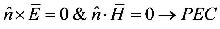 (24)
(24)
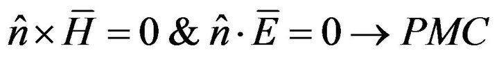 (25)
(25)
It seems that we are at a dead-end, but a new approximation is again proved valid. Explicitly, the normal magnetic field at the surface of a PEC is zero as in (24), but the tangential magnetic field becomes maximum. Hence the relatively small change in the maximum tangential magnetic field caused by substituting PEC with a finite conductivity wall would be negligible. The same is also true for the normal electric field, but we will focus on the tangential magnetic field which is directly involved in the Leontovich boundary condition. On the contrary a similar change in the zero for PEC tangential electric and normal magnetic field would be very significant (Figure 3). The current density flowing on the finite conductivity wall which can be assumed approximately equal to the corresponding surface current density flowing on the PEC wall, which is also defined by 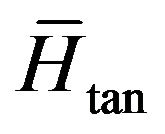 as:
as:
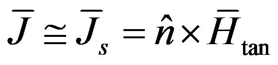 (26)
(26)
Note that the true current density within a finite conductivity conductor is proportional to the tangential electric field 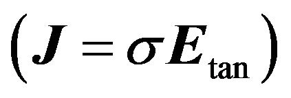 and is thus exponentially reduced inwards from the conductor surface. However, a useful engineering approximation as in (26) assumes an equivalent homogeneous current sheet of thickness equal to the skin depth
  with a value equal to the maximum occurring at its free surface
 . Now, with the availability of a good approximation for
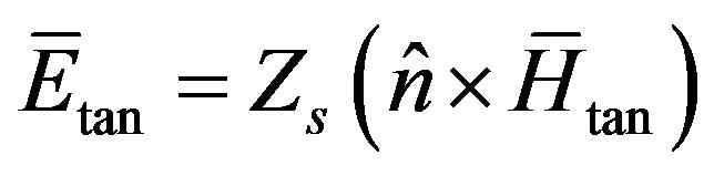
  (Figure 3(b)) the desired
  can be calculated through (16) which can be also written as:
 (27)
(27)
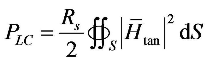
Substituting (26) and (27) into the first term of (23) the conductor losses (PLC) can be estimated solely through the tangential magnetic field from the eigensolution with PEC walls obtained either analytically or numerically as:
 (28)
(28)
where 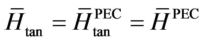 since
since 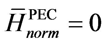 across the PEC wall. Regarding the second term of (23) this can be directly evaluated from the PEC eigensolution, which has already incorporated the complex permittivity and permeability of the material loading. Note that considering complex ε and μ does not add to the problem complexity since a linear eigensystem is retained. Thus the total cavity losses are approximately given by:
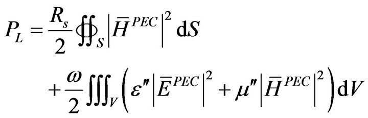 (29)
(29)
The analysis presented above arrives at a very important conclusion: The modal eigenfunction of a practical loaded cavity are approximately the same with those obtained from the eigenproblem with PEC walls and inhomogeneous lossy material loading. These can be exploited for the evaluation of:
• The magnetic Wm and electric We stored energy;
• Both the conductor and material losses through (29);
• The modal quality factors substituting these quantities into (22) or recalling that at resonance 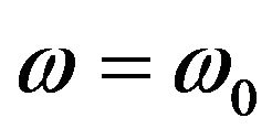 the energy oscillates (one maximized the other vanishes and vice-versa) in time between its electric and magnetic form as
 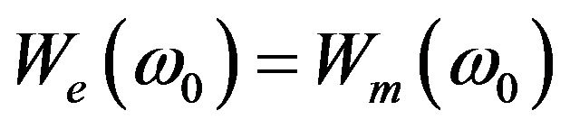 then (22) read:
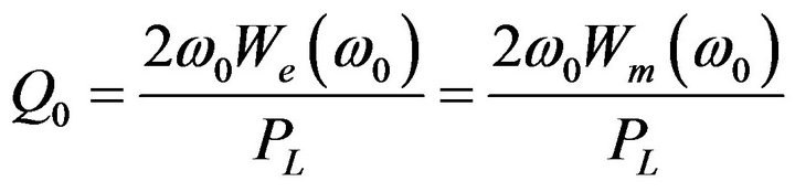 (30)
(30)
Even though classical knowledge is utilized in the above reasoning, a very important conclusion is extracted
 (a) (b)
Figure 3. Electric and Magnetic boundary conditions over a metallic wall with (a) infinite and (b) finite conductivity.
as: “There is no practical need to solve the eigenproblem including the non-linear metallic conductor losses, but all necessary quantities can be approximately extracted from the PEC eigenmode solution”. This is a great simplification since the PEC eigenproblem is linear. On the contrary when conductor losses are incorporated in the formulation through Leontovich impedance conditions it yields a non-linear eigenproblem of fourth order involving  and
and . Solving a linear eigenproblem yields directly the whole eigenspectrum, while the non-linear one requires sophisticated techniques usually based on initial values of a related linear configuration which are iteratively updated. If a non-linear eigenproblem is inevitable, it is preferable to adopt linearization techniques applicable for polynomial forms and this approach is followed next.
3.4. Linearization of the Non-Linear Eigenproblem
In order to solve numerically the Polynomial Eigenproblem (PEP), a transformation into a linear Generalized Eigenproblem (GEP) of larger dimensions (mxn) is applied herein. In general there are two main linearization techniques the companion and the symmetric, but they are not unique for the given problem. The companion linearization is the most used in practice, even though it leads into a non positive definite matrix constituting a serious problem for the solution procedure. For the case of the symmetric linearization there is a lack of GEP techniques that can be applied directly. The standard direct solver fail to manipulate this problem not only due to its size but also due to its ill-conditioning. The main difficulty in the direct solver is the inversion of the right hand side matrix since its determinant vanishes. Thus, the only alternative is the use of iterative solvers, which are in general most efficient especially for large sparse systems of this order, for instance Arnoldi or JacobiDavidson technique. The problem herein is the type of factorization deflation e.g. [16]. Most iterative solvers use a Cholesky factorization, for complex eigenvalue systems, in order to bring the system in an appropriate form before applying the iterative technique and solve it. Due to the fact that in “Leontovich problem” the linearized matrices are not positive definite the Cholesky factorization cannot be constructed. This obstacle can only be overcome using an iterative algorithm with a different kind of factorization. The solution procedure we use is an initial QR factorization and in turn an Arnoldi algorithm with a specific sigma shift, which exploits the sparsity of the matrix system [17].
Examining the form of (19), the polynomial eigenvalue problem can be manipulated with two different techniques. According to the first one the non-linear problem is transformed into an equivalent fourth order linear problem, while according to the second one into an equivalent of second order. These linearization transformations are defined according to Zhu and Cangellaris ([13], pp. 241, 250) as eigenvalue transformation and eigenvector transformation respectively.
3.4.1. Eigenvalue Transformation
The form of (19) can be easily characterized as a fourth order eigenvalue problem, by simply setting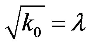 . Thus it can be written in a more general form as:
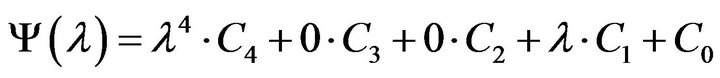 (31)
(31)
where . After the companion linearization the form obtained becomes:
 (32)
(32)
where:
 (33)
(33)
 (34)
(34)
The solution procedure of this kind of problem produces two pairs of complex conjugate eigenvalues of the form:
 (35)
(35)
Only eigenvalue with both real and imaginary positive values can be accepted as representing physical resonant modes. An eigenvalue with negative real part (negative resonant frequency) has no physical meaning and could only be defined as the image of the corresponding positive in frequency domain. The desired complex wavenumber is then calculated as:
 (36)
(36)
3.4.2. Eigenvector Transformation
After a little manipulation formula (19) is reformulated to:
 (37)
(37)
By setting the quantity 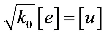 a new eigenvector is introduced and Equation (37) is transformed to:
 (38)
(38)
Assuming now that the quantity  is the eigenvalue, the final system reads:
 (39)
(39)
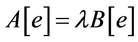
In a compact form can be written as:
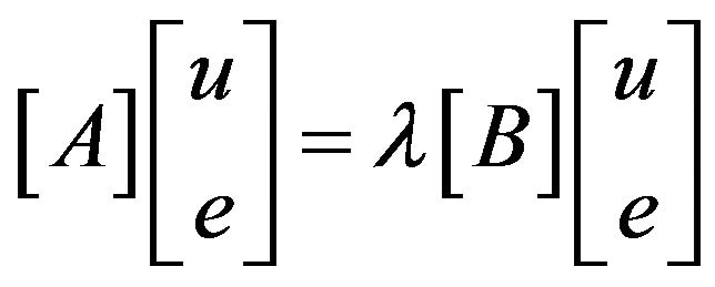 (40)
(40)
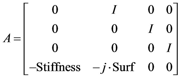
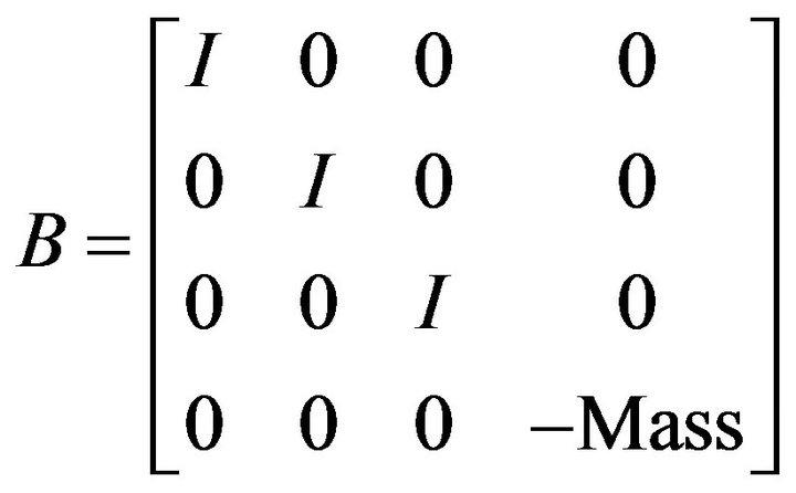
where the matrices A and B are correspondingly:
 (41)
(41)
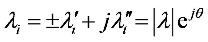
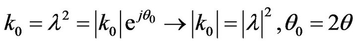
The desired complex wavenumber k0 from the resulting eigenvalue λ is evaluated as:
 (42)
(42)
From the physical point of view  thus
thus  and eigenvalues λ should have both positive real and imaginary parts.
4. Future Extensions
The formulation presented above can be extended to three possible directions with valuable applications. The first refers to a domain decomposition approach but adapted to eigenproblems, in order to address not only the analysis but also the design of large structures based on eigenvalues and numerical eigenfunctions. For example to devise the appropriate antenna, offering the desired field distribution, within an arbitrarily shaped and loaded reverberation chamber. The main idea within this effort is to combine analytically available canonical-subdomain numerical eigenfunctions expansions with numerical eigenfunctions, formulated within complicated subdomains. For this purpose we are in the road toward the establishment of novel orthogonality relations.
The second direction of substantial importance is the eigenanalysis of open-radiating three dimensional structures. A formulation based on the combination of FEM and spherical harmonics is already prepared, but we are facing major computational challenges along with the difficult non-linear character of this eigenproblem. The former challenge can be possibly addressed through a truncation of the boundary integrals in a manner similar to that utilized in Fast Multipole approaches [12]. For the latter challenge numerous approximate linearization techniques are currently considered, starting from an equivalent closed cavity with losses as the one already studied. Note that this could be very useful since the final “global radiation conditions” for the open structure will finally yield an equivalent impedance condition, where the major part of the losses will represent energy leakage through radiation.
The third extension refers to the formulation of an eigenproblem more appropriately suited for the study of radiation phenomena. For this purpose the “internal FEM degrees of freedom” will be eliminated through algebraic manipulations to yield an eigenproblem involving only the outer surface degrees of freedom. This could be characterized as “numerical Green’s functions approach”, since it will provide a complex system matrix similar to that obtained by a Moment Method. The direct eigenanalysis of this complex eigensystem will yield the socalled “complex external eigenmodes”. Besides that, a discrimination of the complex quantities into real and imaginary parts may provide a real valued eigenproblem providing the so called “characteristic modes”, which best describe the structure radiation properties. The strength of such an approach over the traditionally utilized Moment Method lies in the FEM ability to conveniently describe complicated three dimensional structures, e.g. a mobile phone in the neighbourhood of a human head. A possible success of such an approach may open vast new horizons in the “characteristic modes” eigenanalysis. For example, approaches retaining only the degrees of freedom over metallic surfaces will yield electric eigencurrents. Likewise, retaining only certain apertures degrees of freedom may provide a type of magnetic eigencurrents. Both of them can provide valuable analysis and design tools, but mostly will offer the physical insight to devise novel radiators or microwave devices.
5. Numerical Results
Indicative results presenting the capabilities of the above methodologies are given next, while extensive validations and more complete representations can be found in our previous publications specific for each method, e.g. [1-3]. Both the two dimensional and three dimensional finite element analysis techniques were developed in our laboratory from Dr. Allilomes and Mr. Zekios respectively.
5.1. The Hybrid Finite Element Results
An indicative example for the two dimensional eigenanalysis is the leaky wave antenna shown in Figure 4. It consists of a rectangular waveguide with an axial slot, eccentrically located at one of its large walls. A stub or a parallel plate waveguide section is attached to this slot, which ends up to asymmetrical flanges placed at an angle φ. From the engineering point of view the question is to estimate the stub dimensions (a’, c) and the flange angle φ in order to get the desired radiation characteristics. It is by now well established, e.g. [18,19], that these radiation characteristics are uniquely defined by the complex propagation constant of the leaky wave.
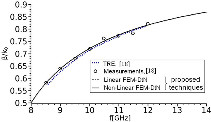
Lampariello et al. [18] have also analyzed this leaky wave antenna using an equivalent Transverse Resonant network (TRE network). In Figure 5 the longitudinal propagation constant is plotted versus frequency, where a very good agreement is observed between the proposed technique and the measurements [18].
Comparing the results with the corresponding of the TRE method an existent mismatch appears. However as it seems, this happens because of the approximate nature of the TRE method which presents a large deviation from the measurements given by Lampariello [18]. Furthermore the agreement between the linear and the non linear FEM-DtN is very good for any frequency of Figure 5.
Let us now present the behaviour of the leaky wave antenna from the engineering point of view. The most
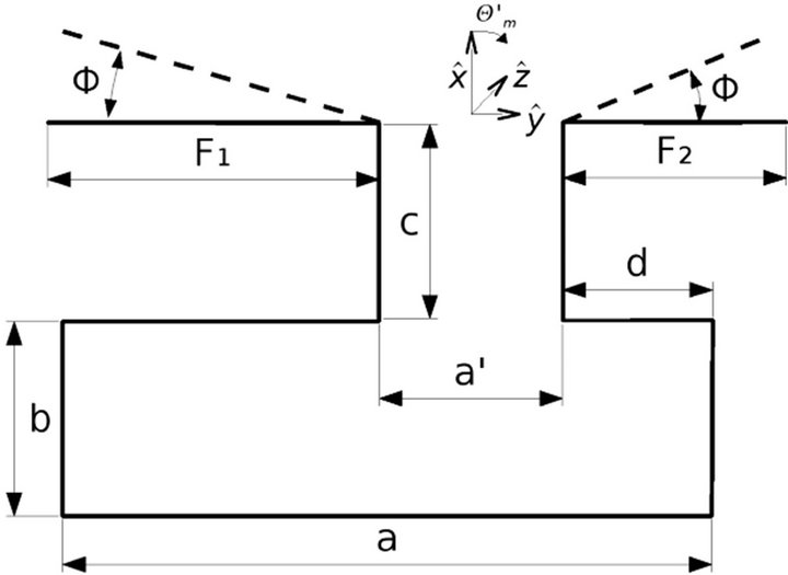
Figure 4. Leaky wave antenna (a = 23.00 mm, b = 11.95 mm, a’ = 11.95 mm, c = 15.64 mm, d = 4.55 mm, F1 = 21.50 mm, F2 = 15.00 mm).
 (a)
(a) (b)
(b)
Figure 5. Normalized longitudinal propagation constant of the leaky wave antenna of Figure 4. (a) Phase constant (β); (b) Leakage constant (α).
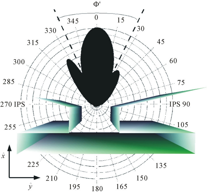
interesting aspect of these types of antennas is to examine the variation of the radiation pattern with respect to the increase of the flanges angles. In Figure 6 a typical radiation pattern of the leaky wave antenna is shown in the case where the two flanges have an arbitrary angle with respect to the main body of the waveguide [18].
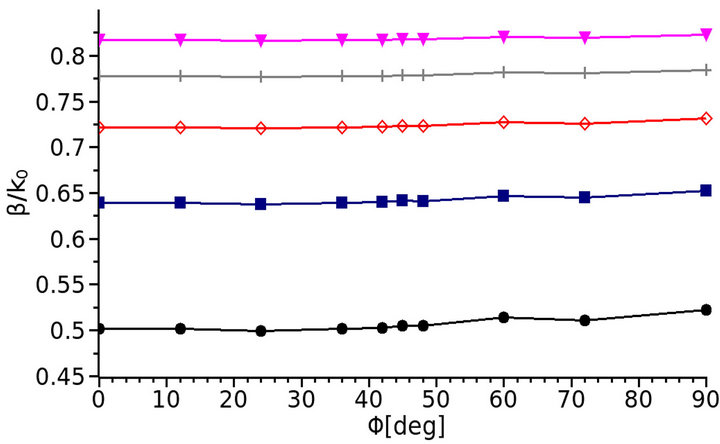
In Figure 7 both the phase (see Figure 7(a)) and leakage (see Figure 7(b)) constants are observed for different flange’s angles and frequencies of 8, 9, 10, 11, 12 GHz. Of critical importance is the fact that the phase constant (Figure 7(a)) is almost constant for the different angles and for every tested frequency. This means that the maximum of the radiation pattern at x-z plane is unchanged in respect to the different flange angles (for more details see Frezza et al. [20,21]). On the other hand studying the leakage constant (Figure 7(b)) there is an increase around the 42˚. The increase of the leakage constant from the
 (a)
(a)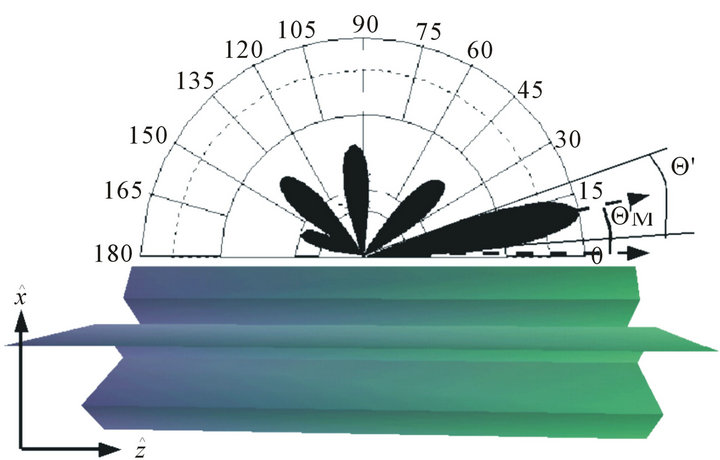 (b)
(b)
Figure 6. A three dimensional view of the leaky wave antenna and typical radiation patterns at (a) x-y plane and (b) x-z plane for the case the two flanges are in an arbitrary angle with respect to the horizontal direction.
 (a)
(a) (b)
(b)
Figure 7. Normalized longitudinal propagation constant versus the angle of the flanges of the leaky wave antenna of Figure 4. (a) Phase constant; (b) Leakage constant.
physical point of view refers to the decrease in the beamwidth of the radiation pattern, thus the increase of the directivity. The reason that the maximum appears at 42˚ and not at 45˚ (at its symmetrical point) is that the two flanges have different lengths. More details are given in the Allilomes’ PhD [22] (in Greek).
5.2. The Resonant Cavity Results
This simulation procedure aims at the overall examination of an electrically large structure. The proposed methodology is validated against analytical solution for the empty cavity and the observed deviation was less than 2% [3]. The topology we study is a reverberation chamber loaded with its main objects (mode stirrer, control base and device under test) as shown in Figure 8. The scope of this test is to examine the variations of the resonant frequencies for an increasing complexity after the successive addition of each object. The mode stirrer produces the main variation of the resonant frequency both in its real and imaginary part. It is a typical cylindrical metallic stirrer consisting of four paddles as shown in Figure 9. The cylindrical axle height is h = 0.1 m and has a radius of r = 0.025 m meters. Each planar scatterer has dimensions l = 0.085 m and w = 0.065 m, while its thickness is d = 0.005 m. The whole structure is metallic and modelled assuming the true finite copper conductiv-
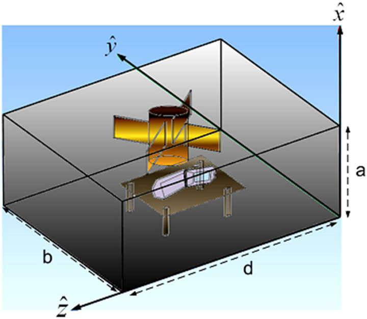
Figure 8. Reverberation Chamber a = 0.2 m, b = 0.4 m, d = 0.5 m loaded with the mode stirrer (given in detail in Figure 9), the control base (0.05 m height) and a mobile phone as the device under test (finite conductivity σ = 58 × 106 S/m).

Figure 9. Metallic (σ = 58 × 106 S/m) mode stirrer with cylindrical axis and four parallelepiped paddles transverse to each other. Typical dimensions gare assumed as: l = 0.085 m, w = 0.065 m, d = 0.005 m, r = 0.025 m, h = 0.1 m, h1 = 0.0175 m, h2 = 0.0175 m.
ity . Table 1 depicts the frequency shift of the first ten resonances with respect to the empty cavity, while Table 2 shows the corresponding quality factor shift. The increase or decrease can be easily explained with the energy change and more specifically with the energy form (electric or magnetic) at the specific position of each scatterer, using the perturbation theory of Section 3.2.
The decrease of the resonant frequencies can be also explained by the example of any ridged waveguide. The introduction of a metallic ridge in a region of maximum electric field decreases the cutoff frequency or the cutoff wavenumber kc and analogously the resonant frequency in cavities, since it is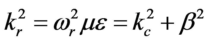 .
.
After the mode stirrer the metallic control base (a table with surface 0.15 × 0.2 m2 and height 0.05 m) is introduced. Recalling that reverberation chambers are utilized for electromagnetic compatibility and immunity testing as well as for MIMO antenna measurements, in all cases the equipment under test (EUT) should be exposed to
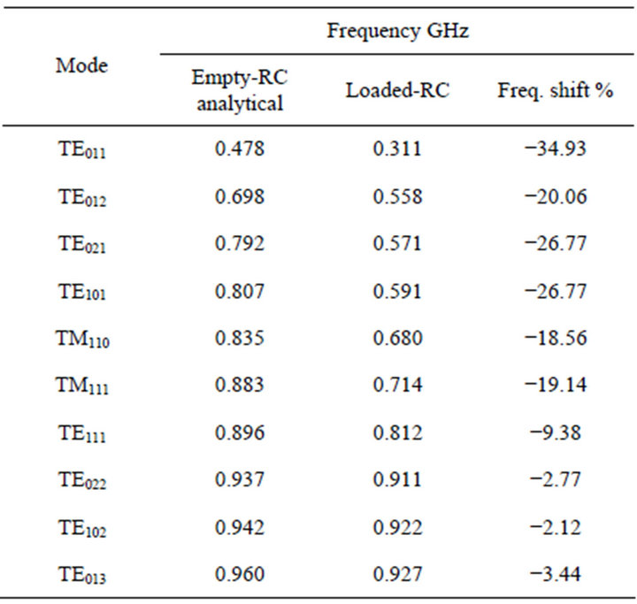
Table 1. Shift in resonant frequencies of the reverberation chamber when loaded with the mode stirrer of Figure 9.

Table 2. Quality factor shift of the reverberation chamber when loaded with the mode stirrer of Figure 9.
maximum and homogeneous field intensity. Hence the EUT should be placed at a location where multiple modes resonating at about the same frequency (to build field at the operating source frequency) present constructive interference. Regarding the horizontal b × d = 0.4 × 0.5 m2 cross section, all odd order modes (TEmnl, TMmnl, ) present field maximum intensity at its center, as shown for example in Figure 10 for the first TE011 mode. Concerning the table height it is more practical for the EUT to be located at the a/4 where even modes present intensity maximum
  while odd modes have significant field concentration.
The resulting variations in resonant frequencies and quality factors are tabulated in Tables 3 and 4 respectively. The table introduction causes some fluctuations in the resonant frequencies along with an additional decrease of the order of 5% - 7% the quality factor due to additional losses.
To accomplish the full simulation for the reverberation chamber the EUT is assumed as a metallic box with dimensions 0.013 m, 0.05 m, 0.11 m (a typical mobile phone), Figure 8. This step is important, since it informs the controller about the frequency response after the introduction of the EUT. This is useful especially for the calibration procedure in practical structures. As shown in
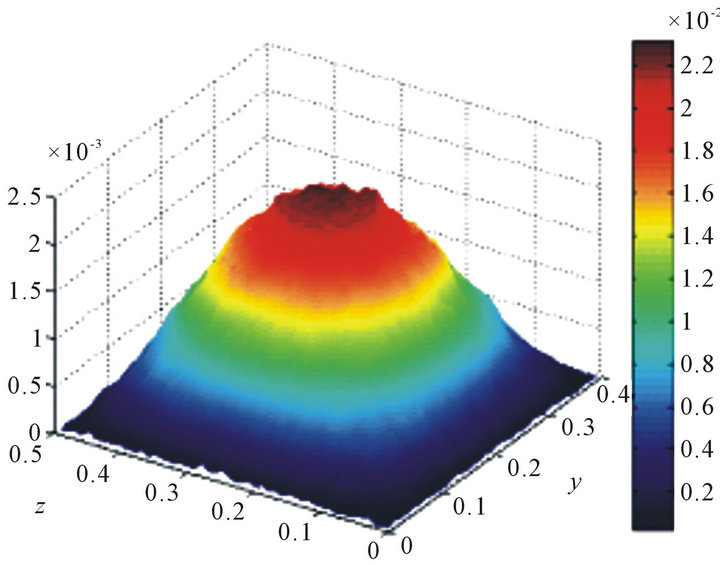
Figure 10. Electric field distribution of the first TE011 mode  over a horizontal cross section at height x = 0.05 m.
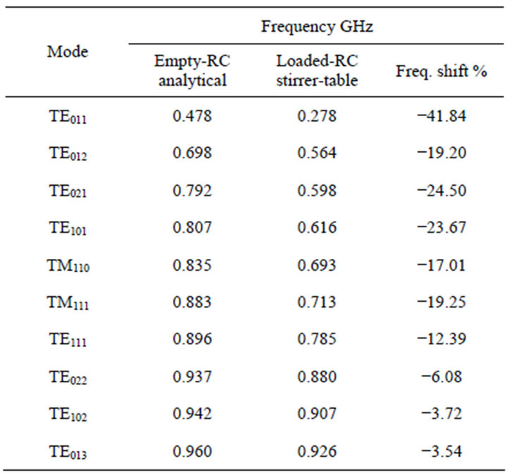
Table 3. Shift in resonant frequencies of the reverberation chamber when loaded with the mode stirrer and the control base.
Tables 5 and 6 respectively, there is no significant shift in the resonant frequencies (less than 2%) nor in the quality factor (less than 3%).
6. Conclusion
A review of an effort on the eigenanalysis of open two dimensional arbitrary shaped waveguides as well as closed three-dimensional electrically large structures is presented. The strengths as well as the limitation of the elaborated methodologies are identified. Indicative nu-
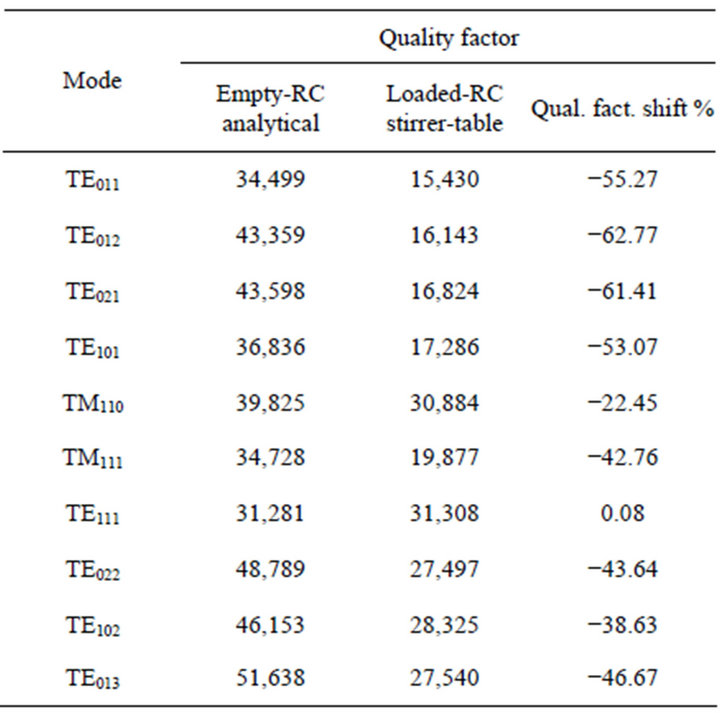
Table 4. Quality factor shift of the reverberation chamber when loaded with the mode stirrer and the control base.
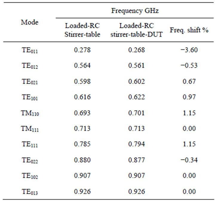
Table 5. Reverberation chamber’s resonant frequencies loaded with the mode stirrer, the control base and the device under test.
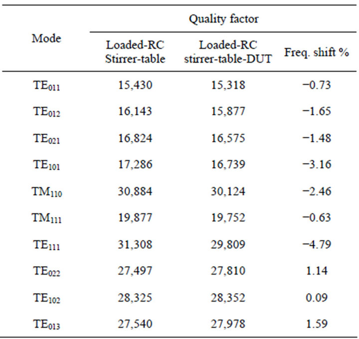
Table 6. Reverberation chamber’s quality factor loaded with the mode stirrer, the control base and the device under test.
merical examples show the capabilities of these methodologies. Possibilities and attractive research challenges calling for the extension of both twoand three-dimensional eigenanalysis are discussed. The extension towards open 3D geometries including characteristic mode eigenanalysis constitutes one of our priorities.
7. Acknowledgements
This research has been co-financed by the European Union (European Social Fund-ESF) and Greek national funds through the Operational Program “Education and Lifelong Learning” of the National Strategic Reference Framework (NSRF)-Research Funding Program: THALES. Investing in knowledge society through the European Social Fund.
REFERENCES
- P. C. Allilomes and G. A. Kyriacou, “A Nonlinear Finite —Element Leaky—Waveguide Solver,” IEEE Transactions on MTT, Vol. 55, 2007, pp. 1496-1510. doi:10.1109/TMTT.2007.900306
- C. L. Zekios, P. C. Allilomes and G. A. Kyriacou, “Eigenfunction Expansion for the Analysis of Closed Cavities,” 2010 Loughborough Antennas and Propagation Conference, Loughborough, 14-15 November 2010, pp. 537-540. doi:10.1049/el.2012.1852
- C. L. Zekios, P. C. Allilomes and G. A. Kyriacou, “On the Evaluation of Eigenmodes Quality Factor of Large Complex Cavities Based on a PEC Linear Finite Element Formulation,” IET Electronics Letters, Vol. 48, No. 22, 2012, pp. 1399-1401.
- D. Givoli, “Numerical Methods for Problems in Infinite Domains,” Elsevier, Amsterdam, 1992.
- D. J. B. Keller and D. Givoli, “Exact Non-Reflecting Boundary Conditions,” Journal of Computational Physics, Vol. 82, No. 1, 1989, pp. 172-192. doi:10.1016/0021-9991(89)90041-7
- J. D. Jackson, “Classical Electrodynamics,” 3rd Edition, Wiley, New York, 1999, p. 431.
- D. M. Pozar, “Microwave Engineering,” 2nd Edition, Wiley, New York, 1998, p. 133.
- C. Reddy, M. Deshpande, C. Cockrell and F. Beck, “Finite Elements Method for Eigenvalue Problems in Electromagnetics,” Tech. Report 3485, NASA, Langley Research Center, Hampton, 1994.
- R. F. Harrington, “Boundary Integral Formulations for Homogeneous Material Bodies,” Journal of Electromagnetic Waves and Applications, Vol. 3, No. 1, 1989, pp. 1- 15. doi:10.1163/156939389X00016
- P. Hager, “Eigenfrequency Analysis: FE-Adaptivity and Nonlinear Eigen-Problem Algorithm,” Ph.D. Dissertation, Chalmers University of Technology, Göteborg, 2001.
- R. Lehoucq, K. Maschhoff and D. Sorensen, “ARPACK Homepage.” http://www.caam.rice.edu/software/ARPACK/
- E. Darve, “The Fast Multipole Method: Numerical Implementation,” Journal of Computational Physics, Vol. 160, No. 1, 2000, pp. 195-240. doi:10.1006/jcph.2000.6451
- Y. Zhu and A. C. Cangellaris, “Multigrid Finite Element Methods for Electromagnetic Field Modelling,” Wiley Interscience, New York, 2006.
- R. F. Harrington, “Time Harmonic Electromagnetic Fields,” IEEE Press, John Wiley and Sons, Inc., New York, 2001.
- Ch. Bruns, “Three Dimensional Simulation and Experimental Verification of a Reverberation Chamber,” Ph.D. Thesis, University of Fridericiana, Karlsruhe, 2005.
- K. Chen, “Matrix Preconditioning Techniques and Applications,” Cambridge University Press, Cambridge, 2005. doi:10.1017/CBO9780511543258
- Y. Saad, “Iterative Methods for Sparse Linear Systems,” 2nd Edition, 2000.
- L. P. Lampariello, F. Frezza, H. Shigesawa, M. Tsuji and A. Oliner, “A Versatile Leaky-Wave Antenna Based on Stub Loaded Rectangular Waveguide: Part III—Comparison with Measurements,” IEEE Transactions on AP, Vol. 46, No. 7, 1998, pp. 1047-1055. doi:10.1109/8.704806
- J. L. Gomez-Tornero, F. D. Quesada-Pereira and A. Alvarez-Melcon, “A Full-Wave Space-Domain Method for the Analysis of Leaky-Wave Modes in Multilayered Planar Open Parallel-Plate Waveguides,” International Journal of RF and Microwave Computer-Aided Engineering, Vol. 15, No. 1, 2005, pp. 128-139.
- E. Frezza and P. Lampariello, “On the Modal Spectrum of the Channel Waveguide,” International Journal of Infrared and Millimeter Waves, Vol. 16, No. 3, 1995, pp. 591- 599. doi:10.1007/BF02066884
- L. P. Lampariello, F. Frezza, H. Shigesawa, M. Tsuji and A. Oliner, “A Versatile Leaky-Wave Antenna Based on Stub Loaded Rectangular Waveguide: Part III—Comparison with Measurements,” IEEE Transactions on AP, Vol. 46, No. 7, 1998, pp. 1047-1055. doi:10.1109/8.704806
- P. Allilomes, “Electromagnetic Simulation of Open-Radiating Structures Based on the Finite Element Method,” Ph.D. Dissertation, Democritus University of Thrace, Greece, 2007.