Applied Mathematics
Vol.4 No.4(2013), Article ID:30369,8 pages DOI:10.4236/am.2013.44087
Hypoexponential Distribution with Different Parameters
1Department of Applied Mathematics, Faculty of Sciences, Lebanese University, Zahle, Lebanon
2Department of Mathematics, Faculty of Sciences, Beirut Arab University, Beirut, Lebanon
3School of Engineering, American University of the Middle East, Eguaila, Kuwait
Email: ksmeily@hotmail.com, therrar@hotmail.com, skadry@gmail.com
Copyright © 2013 Khaled Smaili et al. This is an open access article distributed under the Creative Commons Attribution License, which permits unrestricted use, distribution, and reproduction in any medium, provided the original work is properly cited.
Received January 27, 2013; revised March 4, 2013; accepted March 11, 2013
Keywords: Hypoexponential Distribution; pdf; Convolution; Laplace Transform; Moment Generating Function; Expectation; Partial Fraction Expansion
ABSTRACT
The Hypoexponential distribution is the distribution of the sum of n ≥ 2 independent Exponential random variables. This distribution is used in moduling multiple exponential stages in series. This distribution can be used in many domains of application. In this paper we consider the case of n exponential Random Variable having distinct parameters. Using convolution, some properties of Laplace transform and the moment generating function, we analyse this case and give new properties and identities. Moreover, we shall study particular cases when  are arithmetic and geometric.
1. Introduction
The Random Variable (RV) plays an important role in modeling many events [1,2]. In particular the sum of exponential random has important applications in the modeling in many domains such as communications and computer science [3,4], Markov process [5,6], insurance [7,8] and reliability and performance evaluation [4,5,9, 10]. Nadarajah [11], presented a review of some results on the sum of random variables.
Many processes in nature can be divided into sequential phases. If the time the process spends in each phase is independent and exponentially distributed, then the overall time is hypoexponentially distributed. The service times for input-output operations in a computer system often possess this distribution. The probability density function (pdf) and cummulative distribution function (cdf) of the hypoexponential with distinct parameters were presented by many authors [5,12,13]. Moreover, in the domain of reliability and performance evaluation of systems and software many authors used the geometric and arithmetic parameters such as [10,14,15].
In this paper we study the hypoexponential distribution in the case of n independent exponential R. V. with distinct parameters  for
for  written as
 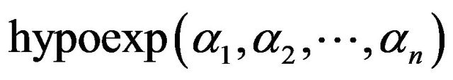 . We use in our work the properties of convolution, Laplace transform and moment generating function in finding the
  derivative of the pdf of this sum and the moment of this distribution of order k. In addition, we deduce some new equalities related to these parameters. Also we shall study the case when the parameters form an arithmetic and geometric sequence considered by [10,14,15] and find some new results.
2. Definitions and Notations
Let  be independent exponential random variables with different respective parameters
 ,
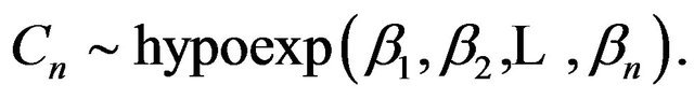
,  , written as
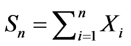
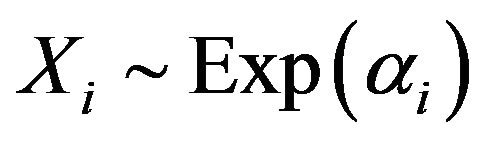 . We define the random variable
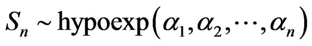
to be the Hypoexponential random variable with parameters ,
,  , written as
Some notations used throughout the paper.
 :
: 
 :
: 
 : The pdf of the random variable X.
 : The cdf of the random variable X.
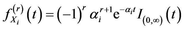
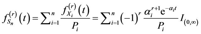
 : The
: The  derivative of the pdf
 .
.
 : Laplace-Stieltjes Transform.
 : Laplace Inverse.
 : The moment generating function of X.
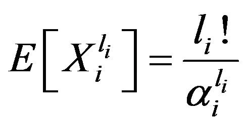
 : The moment of order k of the RV X.
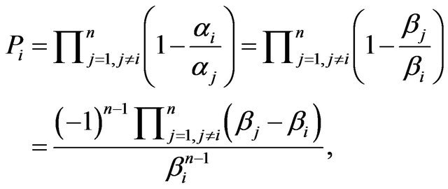
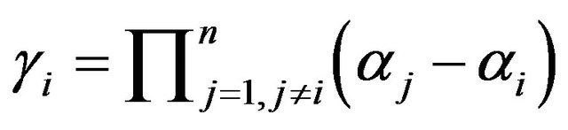
![]() :
:  product of all parameters.
 :
: 
 :
: 
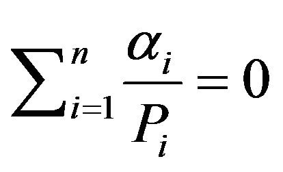
 :
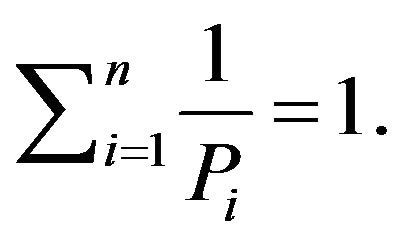
: .
.
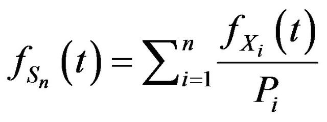
3. Applications on pdf and cdf Using Laplace Transform
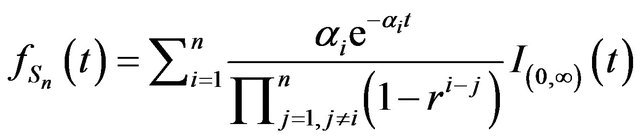
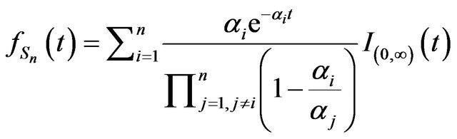
The pdf and cdf of the hypoexponential with distinct parameters were presented by many authors [2,7,11-13]. We shall state in thoerem 1 and propostion 1 these results and provide another proof using Laplace transform. Next, we give some new properties of its pdf, where new identities are obtained.
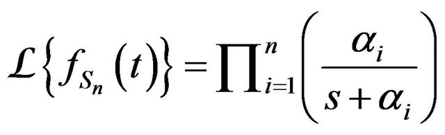
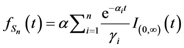
Theorem 1. Let  and
and  Then
Then

and
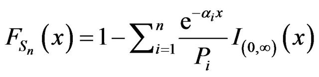 .
.
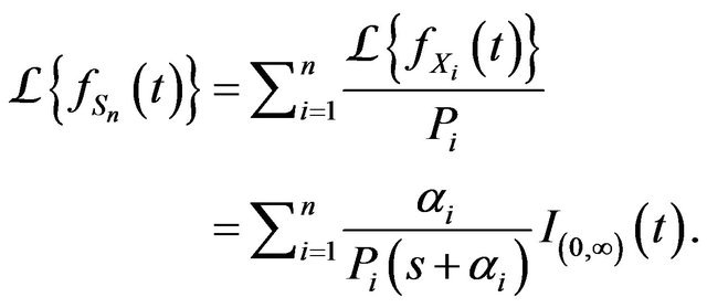
Proof. We have
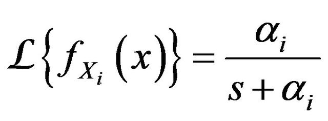 where
where  for
for . Since
  are independent then
  is the convolutions of
 ,
,  written as
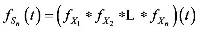
and the Laplace transform of convolution of functions is the product of their Laplace transform, thus
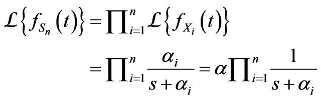 (1)
(1)
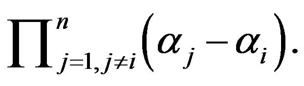
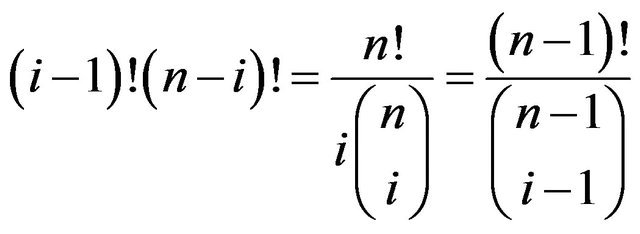
where 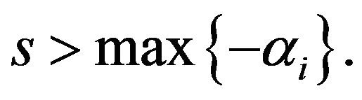 However, by Heaviside Expansion Theorem [16], for distinct poles gives that

where
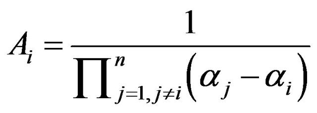 .
.
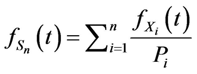
Therefore,
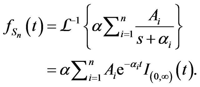
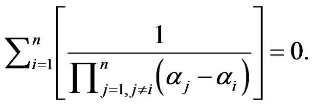
But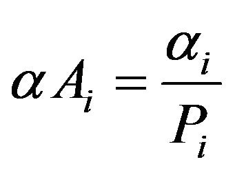 . Thus
 .
.
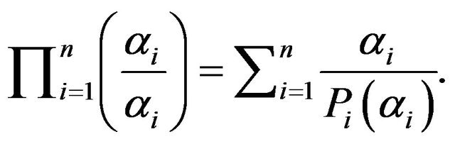
On the other hand we have
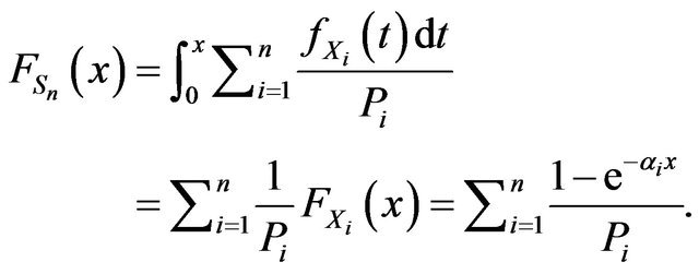
But ![]() then
then 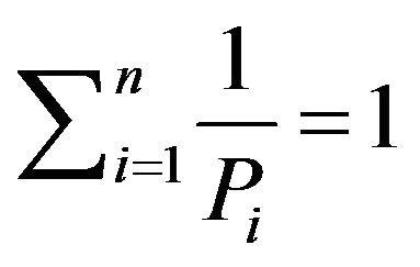 and we conclude that
 .
. 
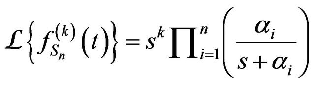
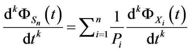
Next we shall discuss the  derivative of
  and many equalities are obtained concerning
  form and some similar forms.
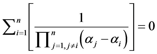
We start by noting from the previous proof that
 . Here, we shall state another simple proof using Laplace transform.
Proposition 1. Let . Then
Proof. We have from Equation (1),
where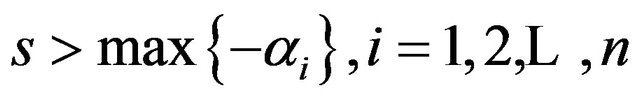 . But from Theorem 1,
and
Hence,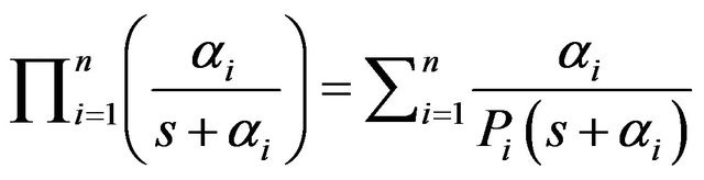 . For
. For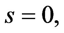
 Therefore,
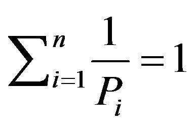 .
. 
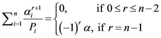
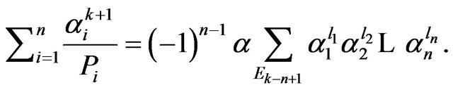
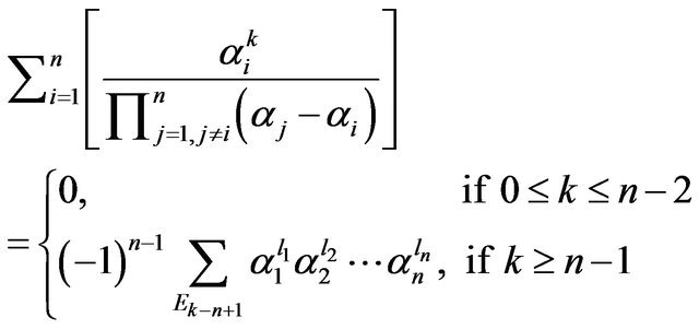
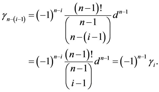
Lemma 1. Let  Then
Then
for 
Proof. The proof is done by induction. For  we have from Equation (1)
 .
.
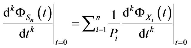
However, by Initial Value Theorem, we have
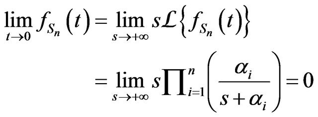
and for  we have
Moreover

Continuing in the same manner till the 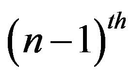 derivative, we obtain the result.
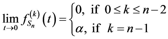
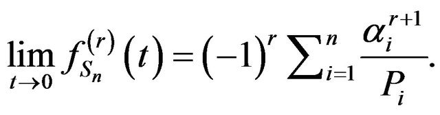
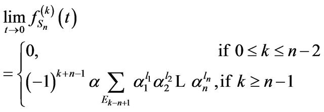
In the following propostion we shall prove that the first  derivative of the pdf of
  are zeros, which verifies the fact that the coefficient of variation of the hypoexponential distribution is less than one unlike the hyperexponential distribution that have the coefficient of variation greater than 1.
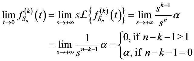
Proposition 2. Let  Then
Then
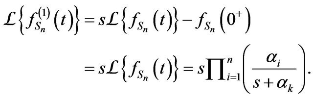
Proof. Let , we have from Lemma 1,

for  and from Initial Value Theorem, we have

Corollary 1. Let . Then

Proof. We have![]() . Then the
. Then the  derivative of
  is
is
 .
.
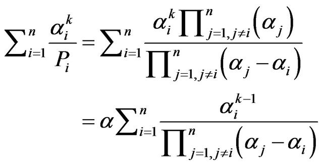
However, from Theorem 1,
 then
then
and
 (2)
(2)
By Proposition 2, we obtain that
By replacing  with
with  we obtain the result.
4. Applications on pdf and cdf Using Moment Generating Function
In the previous section we saw the use of Laplace properties in the proofs of the theorems and propositions. In a similar manner, in this section we use the moment genrating function to obtain more new related results. A new form of the moment generating function of  and the moment of
  of order k is given. Moreover, we deduce more new related equalities concerning
  and higher order derivatives of pdf of
 .
.
Proposition 3. Let  Then
Then
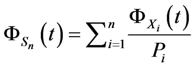 .
.
Proof. We have
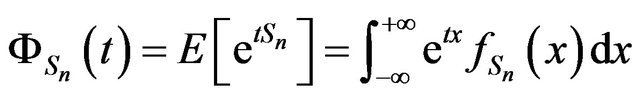
and from Theorem 1,
 then
then
 .
. 
Proposition 4. Let 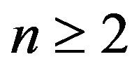 and
and . Then

Proof. We have from Proposition 3,
 .
.
Then
and
which gives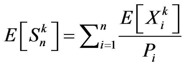 . But
. But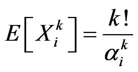 . Thus we obtain the result.
Next, we shall use the Proposition 3 and 4 to find other identities on  and higher orders for
![]() . We start by noting that
. We start by noting that  and by taking
  in Proposition 3, we again obtain the result in Proposition 1that is
 .
.
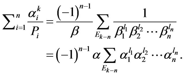
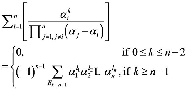
Proposition 5. Let  and
and . Then
where
 .
.
Note that we may write
 , (3)
, (3)
where
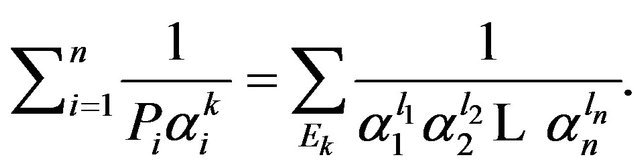
However  and
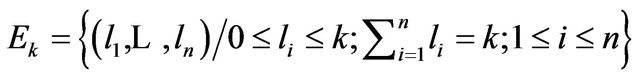
and  are equivalent representing a set of combination with repetition having
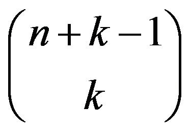
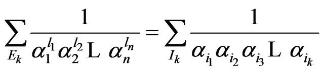
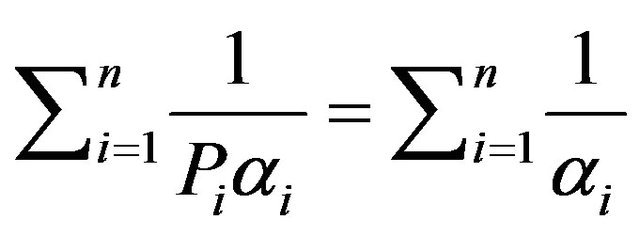
possibilities and , thus the above summation (3) shall be 1.
Proof. Let  and
and . We have
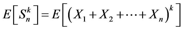
and using multinomial expansion formula, we obtain
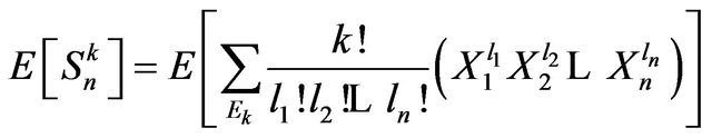 .
.
Knowing that expectation is linear and ,
,  are independent with
 then
then
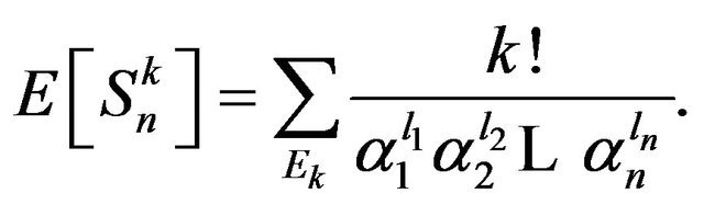 (4)
(4)
Since from Proposition 4,
 .
.
Therefore,
 .
. 
The following corollary is direct consequence of Proposition 5 and Equation (4), taking  and 2 respectively.
Corollary 2. Let . Then 1)
2)  and
and 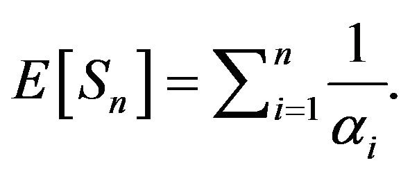
3)  and
and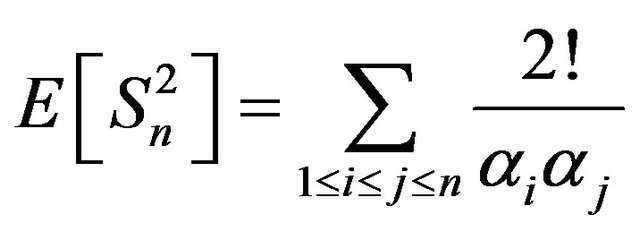 .
.
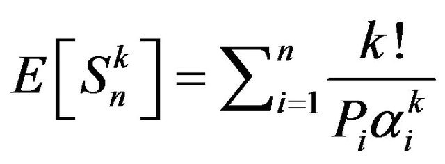
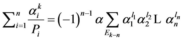
In Proposition 2, we found the first  derivative of
  at 0, However to find higher order derivaties we recall Equation (2), that shows a direct relation between the
  derivative
  and
and . Hence, in the next propostion we shall use Propostion 5, to find an equation for
  by finding a relation between
 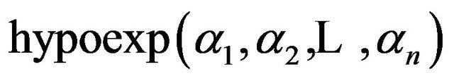 and
and 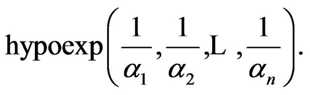
Proposition 6. Let  and
and . Then
Proof. Let 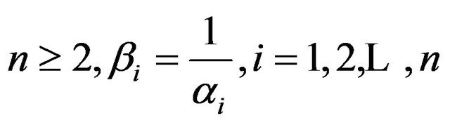 and
and
 Then by Theorem 1, the pdf of
  is
is

where 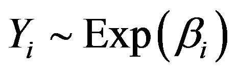 and
and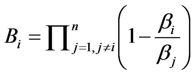 .
.
Next, we shall find  in terms of
 . We have
multiplying in the numerator and denominator by
 we obtain
 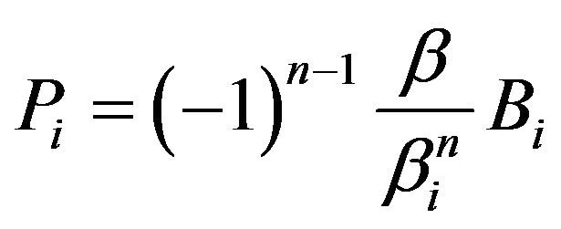 where
where 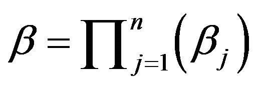 . Hence, we may write
 .
.
But, for  Proposition 5 gives that
 .
.
Therefore,

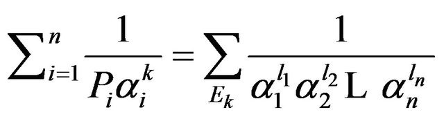
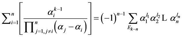
Proposition 7. Let  and
and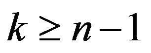 . Then

Proof. We have from Equation (2),

and from Proposition 6,
for 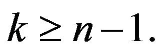 Then,
Then,


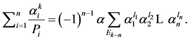
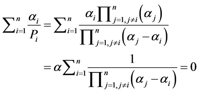
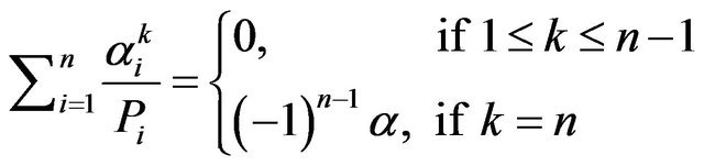
Many authors used the identity
and proved it in many long and complicated methods. Here we shall submit a more simple prove. In addition, we shall find more related identities using the above results.
Proposition 8. Let  Then
Then

Proof. Let . By Corollary 1, taking
 ![]() we have
we have  then
then
 .
.
However,
Therefore,

Next we shall find a more general equality using our previous results.
Proposition 9. Let . Then
Proof. Let . Then,
 (5)
(5)
Suppose that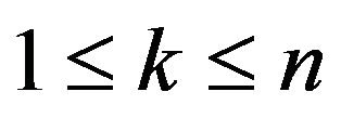 . We have from Corollary 1,
and Equation (5) gives that
Replace  with
with  we obtain the first case and the case when
 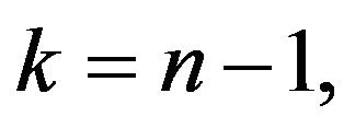 where
where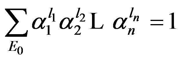 .
.
Now, suppose . By Proposition 6,
and the Equation (5) gives that
 .
.
Also, replace  by
by  we obtain the last case when
 .
. 
5. The Main Results
We summarize Proposition 2 and 7 in the following theorem.
Theorem 2. Let  Then
Then
Also Corollary 1 and Proposition 5 and 6 can be summarized in the following theorem.
Theorem 3. Let  and
and . Then 1)
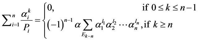
and 2) 
We recall Propostion 9 in the following corollary of Theorem 3.
Corollary 3. Let . Then
6. Case of Arithmetic and Geometric Parameters
The study of reliability and performance evaluation of systems and softwares use in general sum of independent exponential R.V. with distinct parameters. The model of Jelinski and Moranda [14], considered that the parameters changes in an arithmetic sequence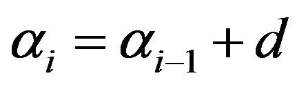 . Moreover, Moranda [15], considered the model when
  changes in an geometric sequence
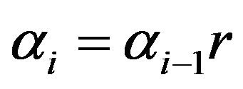 . In this section, we study the hypoexponential in these two cases when the parameters are arithmetic and geometric, and we present their pdf.
6.1. Case of Arithmetic Parameters
We first consider the case when  form an arithmetic sequence of common difference
![]() .
.
Lemma 2. For all 
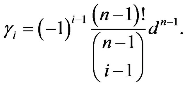
Proof. Suppose that  form an arithmetic sequence of common difference
![]() . Then
. Then 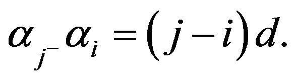 We have
 .
.
Hence,
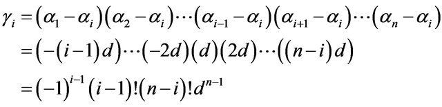
However,
 .
.
Then

Lemma 3. For all 
 .
.
Proof. We have from Lemma 2,
for all  Replace
  by
by , we obtain
Thus we obtain the result. 
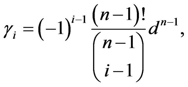
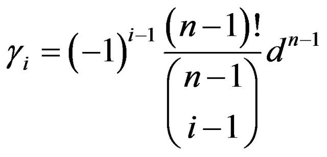
Proposition 10. Let  Then
Then
 where
where

for all 
Proof. We have from Theorem 1

that can be written as
 where
where  and by the Lemmas 2 and 3 we obtain the result.
6.2. Case of Arithmetic Parameters
Next, we consider the case when  form a geometric sequence of common ratio
 .
.
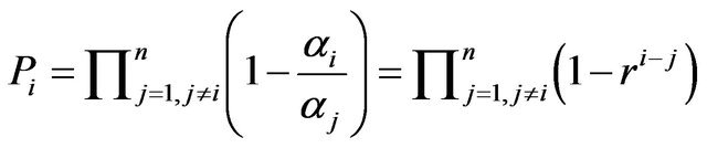
Proposition 11. Let  Then
Then
 .
.
Proof. We have from Theorem 1,
 .
.
Suppose now the parameter  form geometric sequence of common ratio
 . Then
 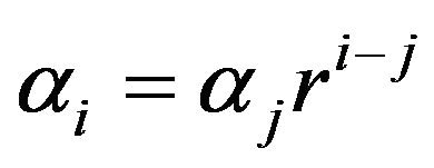 and
and
 .
. 
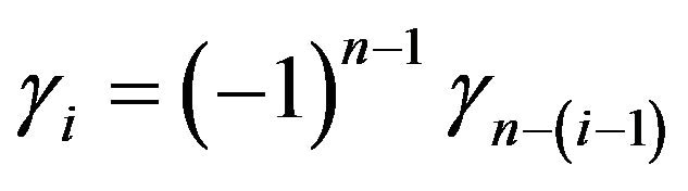
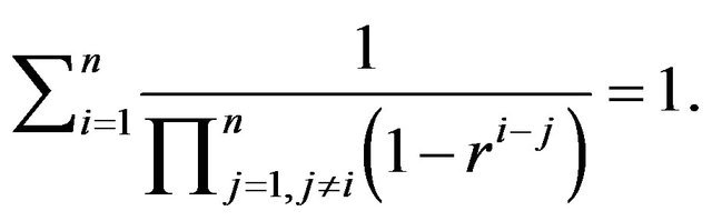
We may also note that the equalities obtained for  represent here a special case and worth mentioning such as
7. Conclusion
The pdf and cdf and some related properties of the hypoexponential distribution with distinct parameters were established. The proofs have been done by using Laplace transform and moment generating function technique. Also with the help of some known computational theorems as Heaviside expansion theorem and multinomial expansion formula the kth order derivative of  and the moment of this distribution of order k were established, in addition for some new related equalities. Eventually, the pdf for models when the parameters
  are arithmetic and geometric were presented. However the other two cases for hypoexponential distribution when the parameters are equal or not all equal can be studied and observed for future studies. It may be checked if they have the same properties as in this paper.
REFERENCES
- W. Feller, “An Introduction to Probability Theory and Its Applications,” Vol. II, Wiley, New York, 1971.
- S. M. Ross, “Introduction to Probability Models,” 10th Edition, Academic Press, San Diego, 2011.
- B. Anjum and H. G. Perros, “Adding Percentiles of Erlangian Distributions,” IEEE Communications Letters, Vol. 15, No. 3, 2011, pp. 346-348. doi:10.1109/LCOMM.2011.011011.102143
- K. S. Trivedi, “Probability and Statistics with Reliability, Queuing and Computer Science Applications,” 2nd Edition, John Wiley & Sons, Hoboken, 2002.
- W. Kordecki, “Reliability Bounds for Multistage Structure with Independent Components,” Statistics & Probability Letters, Vol. 34, No. 1, 1997, pp. 43-51. doi:10.1016/S0167-7152(96)00164-2
- A. M. Mathai, “Storage Capacity of a Dam with Gamma Type Inputs,” Annals of the Institute of Statistical Mathematics, Vol. 34, No. 1, 1982, pp. 591-597. doi:10.1007/BF02481056
- L. D. Minkova, “Insurance Risk Theory,” Lecture Notes, TEMPUS Project SEE Doctoral Studies in Mathematical Sciences, 2010.
- G. E. Willmot and J. K. Woo, “On the Class of Erlang Mixtures with Risk Theoretic Applications,” North American Actuarial Journal, Vol. 11, No. 2, 2007, pp. 99-115. doi:10.1080/10920277.2007.10597450
- G. Bolch, S. Greiner, H. Meer and K. Trivedi, “Queueing Networks and Markov Chains: Modeling and Performance Evaluation with Computer Science Applications,” 2nd Edition, Wiley-Interscience, New York, 2006.
- O. Gaudoin and J. Ledoux, “Modélisation Aléatoire en Fiabilité des Logiciels,” Hermès Science Publications, Paris, 2007.
- S. Nadarajah, “A Review of Results on Sums of Random Variables,” Acta Applicandae Mathematicae, Vol. 103, No. 2, 2008, pp. 131-140. doi:10.1007/s10440-008-9224-4
- M. Akkouchi, “On the Convolution of Exponential Distributions,” Chungcheong Mathematical Society, Vol. 21, No. 4, 2008, pp. 501-510.
- S. V. Amari and R. B. Misra, “Closed-Form Expression for Distribution of the Sum of Independent Exponential Random Variables,” IEEE Transactions on Reliability, Vol. 46, No. 4, 1997, pp. 519-522. doi:10.1109/24.693785
- Z. Jelinski and P. B. Moranda, “Software Reliability Research,” Statistical Computer Performance Evaluation, Academic Press, New York, 1972, pp. 465-484.
- P. B. Moranda, “Event-Altered Rate Models for General Reliability Analysis,” IEEE Transactions on Reliability, Vol. R-28, No. 5, 1979, pp. 376-381. doi:10.1109/TR.1979.5220648
- M. R. Spiegel, “Schaum’s Outline of Theory and Problems of Laplace Transforms,” Schaum, New York, 1965.