Applied Mathematics
Vol.4 No.3(2013), Article ID:28849,8 pages DOI:10.4236/am.2013.43068
The Finite Element Approximation in Hyperbolic Equation and Its Application
—The Pollution of the Water in the West of Algeria as an Example
1Department of Mathematics, Faculty of Science, University of Mohamed Boudiaf USTO, El’ Monour Oran, Algeria
2Hydrometeorological Institute of Formation and Research, Seddikia, Oran, Algeria
3Laboratory of Polymer Chemistry, Faculty of Sciences, University of Oran, Oran, Algeria
Email: saleh_boulaares@yahoo.fr, khaled_mahdi@yahoo.fr
Received January 12, 2013; revised February 12, 2013; accepted February 19, 2013
Keywords: Finite Element; Stability Analysis; Pollution
ABSTRACT
Hyperbolic variational equations are discussed and their existence and uniqueness of weak solution is established over in the last six decades. In this paper the hyperbolic equations (strong formula) can be transformed into a Hyperbolic variational equations. In this research, we propose a time-space discretization to show the existence and uniqueness of the discrete solution and how we apply it in the transport problem. The proposed approach stands on a discrete L∞-stability property with respect to the right-hand side and the boundary conditions of our problem which has been proposed. Furthermore the numerical example is given for the pollution in the smooth fluid as water and we have taken the pollution of the water in the west of Algeria as an example.
1. Introduction
The construction of a numerical model consists of two distinct stages: the first is to establish a system of equations and strongly coupled nonlinear governing the behavior of continuous phenomena.
In the late 40’s methods of grid points were used to model the universally large-scale atmospheric flow. During recent years, alternative methods have been used, one of these methods is the finite element method finis. In this paper, we present the main tools for implementations of the method more generally belong to family of Galerkin methods. These are commonly used instead of the finite difference method (considered too simplistic) to treat horizontal and vertical fields in the models.
Galerkin methods, which can solve numerically systems of equations and inequalities PDE (see ref. [1,2]) do not directly use the field values at the points of a grid, but are use of series expansions of functions appropriately chosen, so as to reduce the resolution of a system of ordinary differential equations. There are two types of methods within this process: the finite element method for which the functions are zero, except for a small area where they are equal to the low-order polynomials, and the spectral method in which the functions are the functions of a spatial operator defined on the entire work area.
The finite element method is one of the tools of applied mathematics. It is put in place, using principles inherited from the variational formulation or weak formulation, a discrete mathematical algorithm for finding an approximate solution of a free boundary problem (see [3-7]). It speaks Dirichlet conditions (values at the edges) or Neumann data. The finite element method is different than the spectral method because it is not comprehensive, but rather determined by local values. However, it is distinct approximations the function is defined over the entire region and not just the discrete points (see [2]).
The outline of the paper is as follows. In Section 2, we lay down some notations and assumptions needed through out the paper. Moreover, we study a priory estimates of the semi-discrete and prove the stability analysis of finite element for Hyperbolic equation (HE). In Section 3, we associate with the discrete HE problem a main theorem and use that in proving the existence of unique discrete solution. Finally, in Section 5, we applied this method to the equation of transport and its application in the certain pollutants, where the numerical example is given for the pollution in the smooth fluid as water and we have taken the pollution of the water in the west of Algeria as an example.
2. Finite Element Methods for Hyperbolic Equations
2.1. The Classic Formulation
Consider the following problem, hyperbolic first order, in the interval 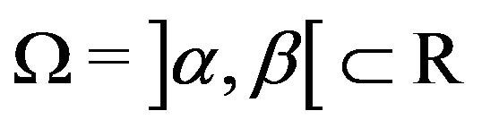
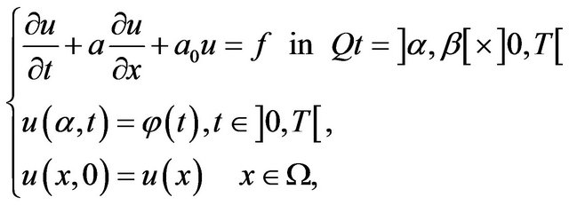 (1)
(1)
2.2. The Variational Formulation
The Continuous Problem
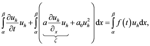
We multiply (1) by  and integer in
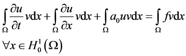 (2)
(2)
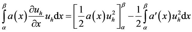
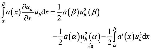
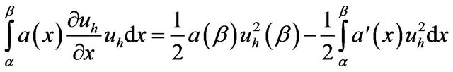
Using the Green formula we have
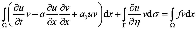 (3)
(3)
the problem becomes:
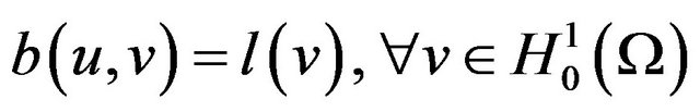
 (4)
(4)
with
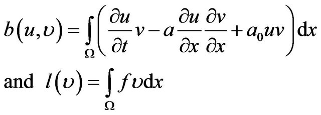
To ensure the existence and uniqueness of the solution we must have:
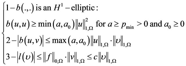
(5)
According the Lax.Milgram theorem, the problem (3) has a unique solution.
3. The Discrete Problem
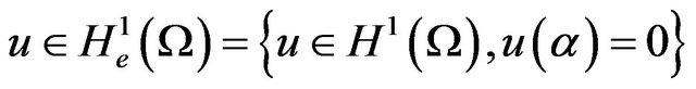
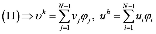
The finite element method is a special case of the variational approximation method, also called the method of Rayleigh-Ritz or Galerkin approach which allows the solution u as follows. We construct a subspace  of finite-dimensional space
 , then we define the approximate solution
  of the solution
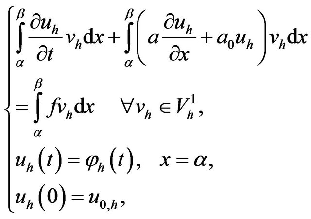
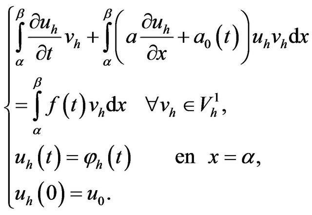
  as the solution to the following problem: Find
  solution of
 (6)
(6)
where
 (7)
(7)
3.1. The Space Discretization
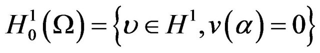
We defined the following space:
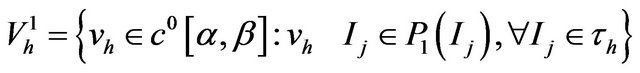 (8)
(8)
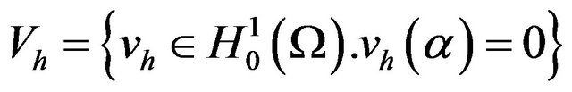 (9)
(9)
we have
 (10)
(10)
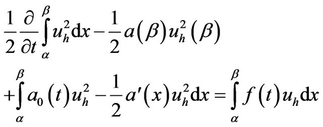
3.2. Existence and Uniqueness of the Solution
We have
 (11)
(11)
we can set , we get
 (12)
(12)
Then

Thus
Then
Equation (12) becomes
 (13)
(13)
We set
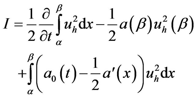
and
We can write (13)
 (14)
(14)
We suppose
 (15)
(15)
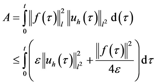
Using the inequality of young
 (16)
(16)
we can write
and
Using (15) we have
and
One integer on 
Then
thus
or
implies
Then
 (17)
(17)
By Using the inequality of Cauchy Schwarz
Using Young inequality
we put . Then
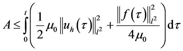
(3.12) equivalent
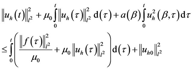
thus, we have
in particular cases or  and
and  are null
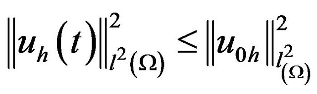
which reflects the stability of the energy of the system.
3.3. The Time Discretization
The time discretization of the finite element methods introduced in the previous section can be done either by finite differences or by finite elements.
If we choose a finite difference scheme implicit, both methods are unconditionally stable.
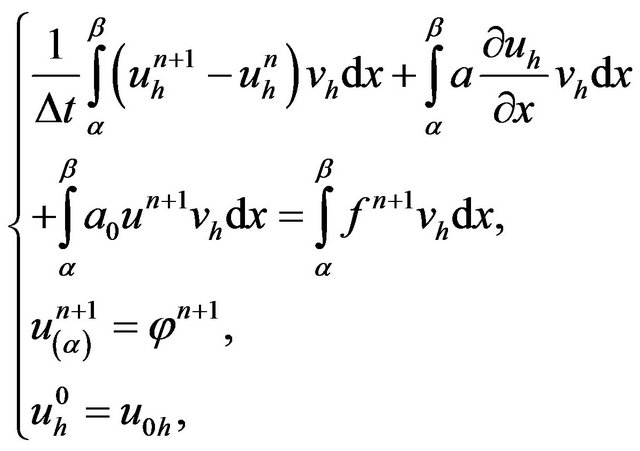
For example, using the implicit Euler method for the time discretization of the problem (3.7). The problem can be written, for all : find
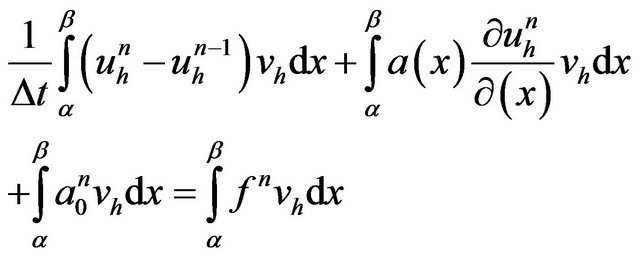 (E)
(E)
with  et
et  if
if  and
and  we set
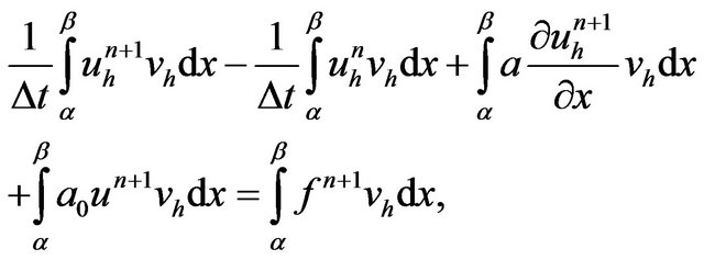
  in (E) we find
 (E1)
(E1)
 (E1)
(E1)
calculation of 
thus, we have
Using 
Then, we deduce
 (18)
(18)
Summing from  to
to , we find, for
In particular, we can conclude that
The diagram is clear, however, subject to a stability condition: for example, in the case of the Euler method, the stability condition is  This restriction is not as severe as in the case of equation parabolic equation. this is particularly why the explicit schemes are used in the approximation of hyperbolic equation.
3.4. Matrix Form
A thorough analysis of the stability and convergence properties of the discontinuous Galerkin method can be found in Thomee (1984), Eriksson, Johnson and Thornee (1985) (see also Dupont (1982)). Let us just recall that the method is formally of order  at the nodal points tn, and of order
  in the global interval
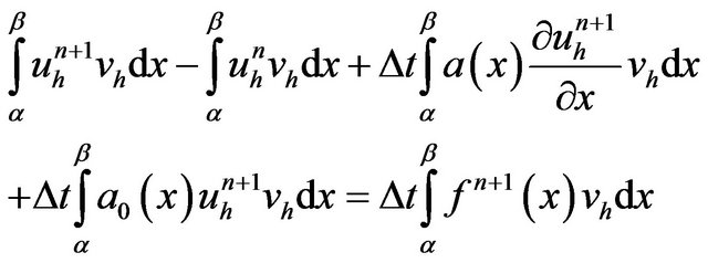
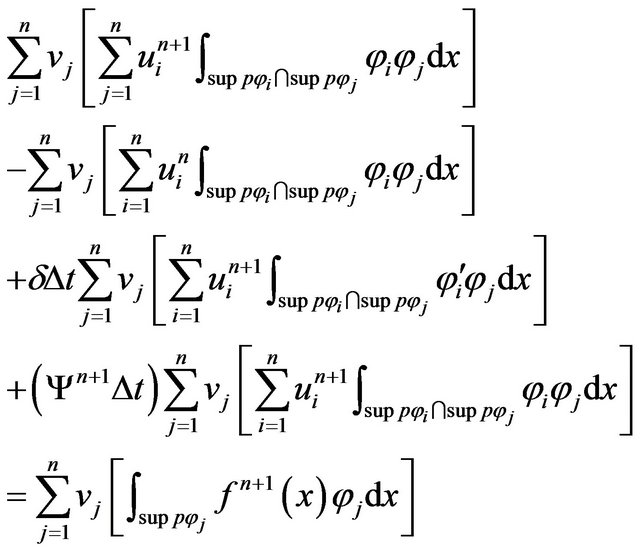
 Now we
 (19)
(19)
thus
or
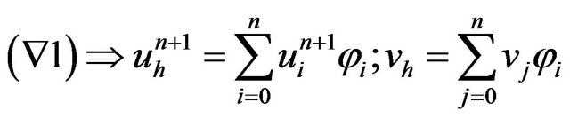
We can write
 (
( 1)
1)
and we have
we set
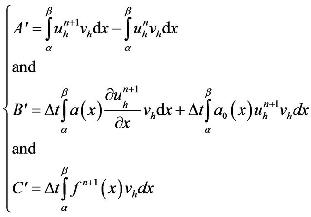
Using
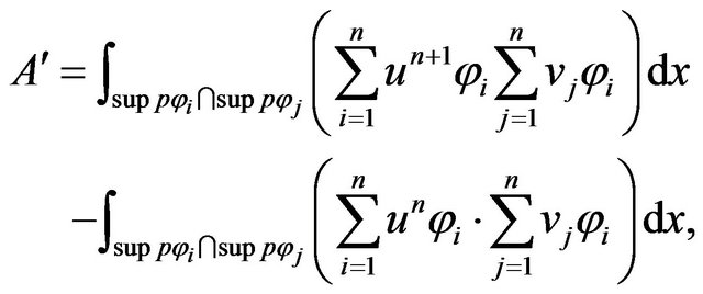
and
with
we consider
The previous relation becomes
and
thus the equation  equivalent
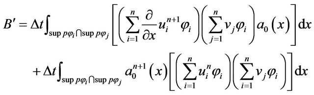
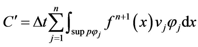
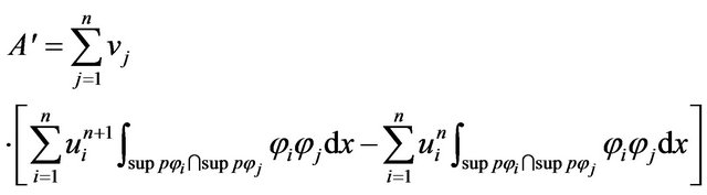
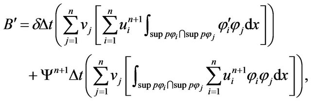
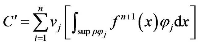
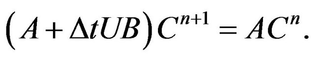
So the above equation to give
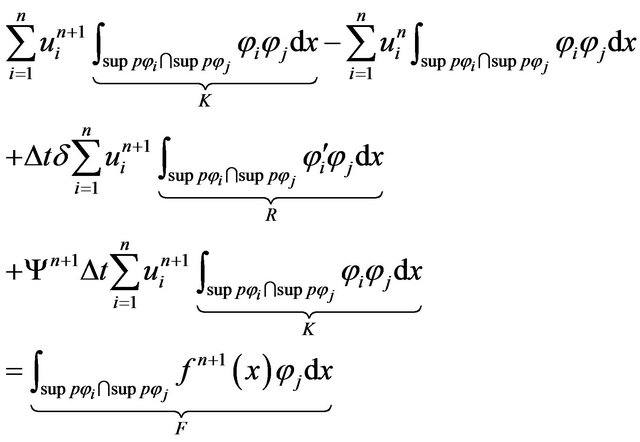
(20)
Our system is reflected in the form:
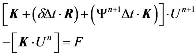 (21)
(21)
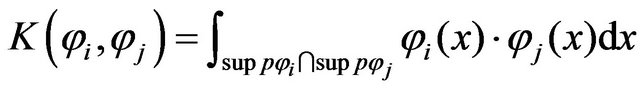
where
-The  symmetric three-diagonal matrix of dimension
  defined as
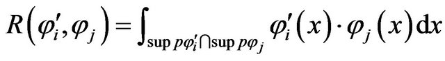
-The matrice  symmetric three-diagonal matrice of dimension
  defined as
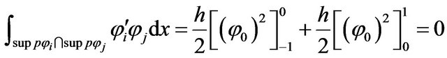
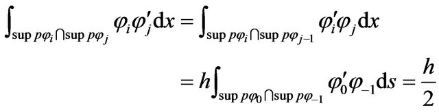
Calculation of the matrices terms
 :
:
1st Case 
Then, we have for
 (22)
(22)
for: 
and for
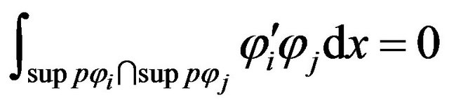 (23)
(23)
2nd Case
We have for 
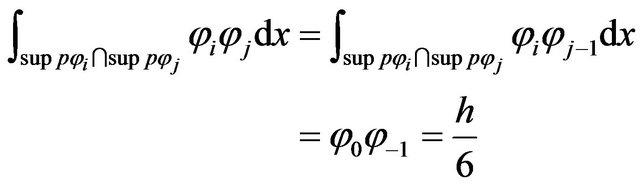
thus we have 
 (24)
(24)
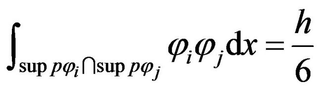
Thus, we have for 
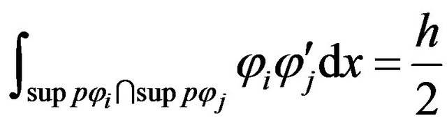 (25)
(25)
3rd Case
For 
 (26)
(26)
and for
 (27)
(27)
4. Application
The dimensional models are developed to assess the phenomena of dispersion in the far field zone wherein the concentration of the released product is homogeneous across the section.
Based on simplifying assumptions including neglecting dispersion phenomena vertical and transverse and longitudinal dispersion. Transport the pollutant is given by the following equation:
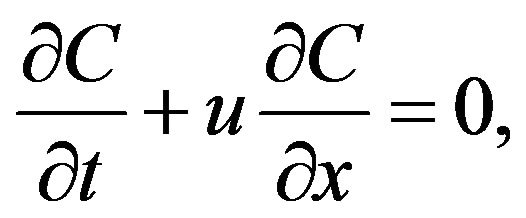 (28)
(28)
with C: concentration of pollutant (mg/L);
U: flow velocity (m/s);
for the application of our model, we chose the site of Wadi EL Meleh (in the west of Algeria).
The watershed of Oued El Maleh is located in the north part of the country in wilaya Ain Témouchent. It is characterized by a Mediterranean climate arid to semiarid with hot influences the Sahara to the south and cold north and east.
This area is known by low rainfall with an average inter-annual 300 mm/year.
The study watershed is located in north-western Algeria is approximately ( and
and ) and between longitude (
 and
and ) latitude.
It is bordered by the Mediterranean Sea to the north, the mountains of Berkeches south, the mountains of El Sbaa Chioukh South West, Tessala Mountains in the South East, Mlata plain to the east and the basin of Ouled El Kihel West (in the west of Algeria).
4.1. Problematic
Equation (28) is a hyperbolic equation, then it would be wise to use a semi-explicit scheme time discretization. We will use the finite element method for discontinuous Galerkin spatial discretization.
The assumptions are:
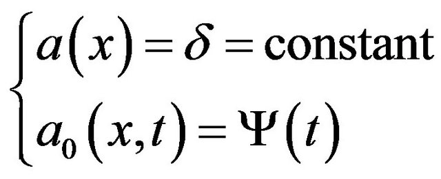
*The velocity is constant and independent of time;
*The density of the pollutant is equal to that of water;
*The pollutant concentrations depend only on time and distance;
*Knowledge of initial conditions and boundary conditions.
4.1.1. The Initial Condition
Considering that the concentrations are zero regardless of the distance downstream of the sampling point.
4.1.2. Boundary Conditions
It is defined by:
*The pollutant is considered conservative or passive, and the principle of conservation of mass is taken into account:
*Concentrations are considered zero after an infinite distance downstream from the point of sample collection:
such that:
A: section of the river (m2);
C: concentration of pollutant (mg/L);
M: mass rejection (Kg).
Calculated flow velocity is given by the following formula:
 (29)
(29)
such that:
S: mesh section (m2);
U: flow velocity (m / s);
Q: average daily flow of the river (m3/s).
The choice of using one-dimensional models can be detrimental in terms of the accuracy of predictions since several phenomena have been neglected. However, the interest lies in the small number of data required making a tool in line with the issue of emergency.
Data.
4.1.3. Hydrodynamic Data
Flood discharge (m3/s)—wet section (m2) main floodlength (m)—Raw slope (m/m)—high flood.
(source station hydrology Turgot North ‘Ain Timouchent).
4.1.4. Choice of Pollutants
Our choice fell on two pollutants: NO2 and NH4 have a large dilution in water, and its harmfulness and toxicity to living beings, in addition to the stream is infected discharges from a manufacturing plant detergents. The manufacture of detergents is based on products of this type.
For this, the laboratory service of the National Agency of Water Resources (ANRH) performs measurements of the chemical composition of the water regularly and in different places.
4.1.5. Explanation
Equation for the program you must enter the input parameters (according to our assumptions):
Insert the U velocity calculated using the formula in Section 4 [u = Q/S].
Insert the  and h = 2 m [h = max hi]. these two parameters are chosen arbitrarily (the semiimplicit time discretization scheme) because it is unconditionally stable. For a maturity de 12 h, we obtain 72 iterations.
Introduction of a number of points: our choice was focused on 5 points due to the low concentration of the pollutant treated to avoid that other phenomenon outweighs the transportation Read initial data from the file container (The data are from the original collection of 16 November 2009 to 08: 35 h).
Matrices are calculated discretization of the array formula defined before
The result was a system of equations to be solved, where  is the forecast (the unknown).
The results of the model are presented in the following graphs (Figure 1).
4.1.6. Comment
The graphs (see the Figure 1) show the temporal evolution of pollutant concentrations  and
and  at differing distances.
We chose a flow velocity of 0.64 m/s because higher speeds cause greater dilution, and therefore very low concentrations.
Diffusion was eliminated and is interested only in the advection.
5. Conclusion
In this paper, we have a new discretization for the finite element approximation of the hyperbolic variational equations and we set the transport equation as model. We have established a convergence and the stability of this equations type, using by the semi-implicit time scheme combined with a finite element spatial approximation. this discretization types, which we get here, is important
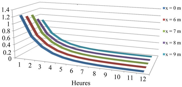
Figure 1. Concentration of NO2 (mg/l).
for the calculus of quasi-stationary state for the simulation of the pollutions concentration for each gaseous. The proposed discretization stands on a discrete  - stability property with respect to the right-hand side and the boundary conditions of our problem which was proposed. Furthermore the numerical application in certain gaseous for our discretization is given and deficient. A future work, we will complete of this research and we will be devoted to the computation and comparison between our discretization and an economic societies data.
REFERENCES
- A. Quarteroni and A.Valli, “Numerical Approximation of Partial Differential Equations,” Springer Series in Computational Mathematics, Springer, Berlin and Heidelberg, 2008. doi:10.1007/978-3-540-85268-1
- H. M. Duwairi and A. Rablhi, “Fluid over a Vertical Surface,” International Journal of Fluid Mechanics, Vol. 32, No. 1, 2005, pp. 81-87. doi:10.1615/InterJFluidMechRes.v32.i3.10
- J. Z. Jordan, “Network Simulation Method Applied to Radiation and Viscous Dissipation Effects on MHD Unsteady Free Convection over Vertical Porous Plate,” Applied Mathematical Modeling, Vol. 31, No. 9, 2007, pp. 2019-2033. doi:10.1016/j.apm.2006.08.004
- S. Boulaaras and M. Haiour, “L∞-Asymptotic Behavior for a Finite Element Approximation in Parabolic QuasiVariational Inequalities Related to Impulse Control Problem,” Applied Mathematics and Computation, Vol. 217, No. 3, 2011, pp. 6443-6450. doi:10.1016/j.amc.2011.01.025
- S. Boulaaras and M. Haiour, “A New Approach to Asymptotic Behavior for a Finite Element Approximation in Parabolic Variational Inequalities,” ISRN Mathematical Analysis, Vol. 2011, 2011, Article ID: 703670. doi:10.5402/2011/703670
- S. Boulaaras and M. Haiour, “The Finite Element Approximation of Evolutionary Hamilton-Jacobi-Bellman Equations with Nonlinear Source Terms,” Indagationes Mathematicae, Vol. 24, No. 1, 2013, pp. 161-173. doi:10.1016/j.indag.2012.07.005
- M. Haiour and S. Boulaaras, “The Finite Element approximation for a Class of Parabolic Quasi-Variational Inequalities with Non Linear Source Terms,” International Journal of Numerical Analysis and Application, Vol. 5, No. 1, 2011, pp. 123-139.