Modern Economy
Vol.4 No.1(2013), Article ID:27597,7 pages DOI:10.4236/me.2013.41006
Testing the Long Run Neutrality of Money in Developing Economies: Evidence from EMCCA
Department of Economics, Omar Bongo University, Libreville, Gabon
Email: ekomie@refer.ga
Received November 9, 2012; revised December 10, 2012; accepted January 10, 2013
Keywords: Long Run Money Neutrality; EMCCA Countries; Unit Root; ARIMA Methodology
ABSTRACT
We examine the long run neutrality of money (LMN, hereafter) in the Economic and Monetary Community of Central Africa (EMCCA) countries, applying Fisher and Seater (1993) Autoregressive Integrated Moving Average (ARIMA) methodology, using different monetary aggregates, money supply in the strict sense (M1), money supply in the large sense (M2) and domestic credit (credit to private sector) during the period 1978-2008. Tests consistently reject the LMN hypothesis. It is found that monetary aggregates have significant and positive impacts on real Gross Domestic Product (GDP) for all EMCCA countries. The results are robust under various sub-periods and the estimated coefficients are stable under two breakpoints corresponding to the dates of central bank reforms and devaluation of the local currency.
1. Introduction
The old debate on the effects of monetary policy on real and nominal variables is experiencing a resurgence of interest with the controversy surrounding the role of central banks. The most widely shared position today is the long run neutrality of money (LMN, hereafter). Literature distinguishes the LMN and the super long-run neutrality of money (LMSN, hereafter). Under the LMN hypothesis, a permanent change in the level of money supply has no impact on the level of real variables in the long run; while the LMSN hypothesis claims that a permanent change in the growth rate of money supply does not affect the level of real variables in the long run.
To test the hypothesis of neutrality of money, Fisher and Seater (1993), King and Watson (1997) respectively use an ARIMA model and the VAR methodology with time series for real output and monetary aggregates. According to these works, two important properties must be met for testing LMN: the exogeneity of money and the non-stationarity of real and monetary variables. Based on annual data from the USA for the period 1865-1975 and monthly data for Germany over the period of hyper-inflation after World War I, Fisher and Seater (1993) argue a weak neutrality of money in the case of the USA and refute the hypothesis of LMSN in the case of Germany [1]. King and Watson (1997) consider the American experience of post-war period from 1949:Q1 to 1990:Q4. Tests reject neutrality and little evidence of LMSN [2].
In addition, Weber (1994), Serletis and Koustas (1998), Leong and McAller (2000), Shelley and Wallace (2006) study the LMN considering the order of integration of variables for industrialized countries [3-6]. However, their results do not provide consensus either in favor or against LMN.
Studies on LMN in emerging countries are relatively rare. Wallace (1999), Bae and Ratti (2000), then Sulku (2011) verify the LMN hypothesis, respectively, in the case of Mexico (1932-1992 period), Brazil and Argentina (1884-1996 and 1912-1995 periods) and Turkey (1987: Q1-2006:Q4), using the methodology of Fisher and Seater (1993) [6-8]. Similarly, Chen (2007) tested the LMN hypothesis in South Korea and Taiwan using King and Watson (1997) methodology. He uses quarterly data from 1970 to 2004 for South Korea and from 1965 to 2004 for Taiwan. Chen (1997) finds strong support for the LMN in the case of South Korea but poor evidence in favor of the LMN in the case of Taiwan [9].
Although there are relatively numerous studies investtigating the LMN for developed countries as well as emerging economies, the literature on developing countries is emerging and is still at its earlier stage.
In this paper, we would like to contribute to the development of the literature on LMN for African countries, building on the Economic and Monetary Community of Central African (EMCCA) countries case. These countries have in common a Central Bank, the Central African States Bank (CASB) whose primary mission is monetary stability. This means price stability and a sufficient level of foreign exchange reserves, as the local currency (CFA francs) is linked to the European currency (the Euro). Therefore, the LMN is necessary for the success of monetary stability strategy. That is why, testing the LMN for EMCCA countries becomes even more attractive and important.
The study is based on the Fisher and Seater (1993) ARIMA methodology not only because it is appropriate but also for its simplicity. Even though our period of study is relatively short, as explained in Fisher and Seater (1993), since there were sudden changes in money and prices, this data set is qualified to be used for controlling a long run relationship.
The remainder of the paper proceeds as follows: Section 2 established the LMN and LMSN based on the Fisher and Seater’s (1993) methodology. In Section 3, our data set is introduced. Empirical results are presented and discussed in Section 4. Some concluding remarks appear in Section 5.
2. Econometric Methodology
2.1. LMN and LMSN in Fisher and Seater’s (1993) ARIMA Methodology
Fisher and Seater (1993) consider a system of log linear, stationary and invertible ARIMA model of two variables. The following model of the log of money supply  and the log of real GDP
  has been demonstrated,
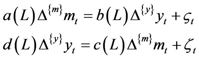 (1)
(1)
where  and
and  are the orders of integration of the money supply and the real GDP respectively. The vector
  is independently identically distributed with zero mean and the covariance
  which is composed of
  and
and .
.
If we consider the specific case when 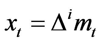 and
and 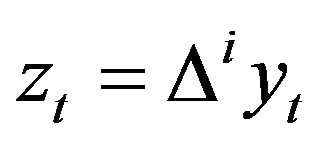 such that
  and
and  are equals to 1 or 0, then the long run effect of permanent change in
  on
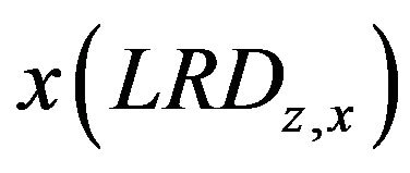
on  is equal to the long run derivative of
  with respect to
 ,
,
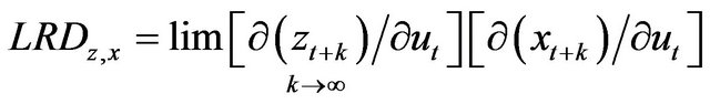 (2)
(2)
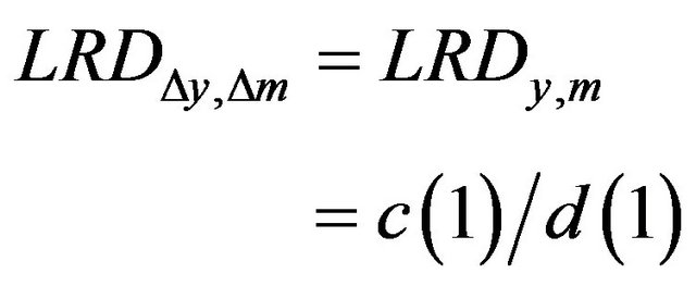
As stated in Fisher and Seater (1993), if
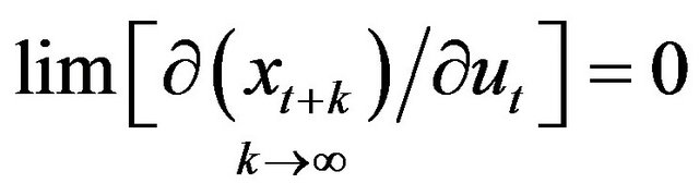
then there are no permanent changes in monetary variables, so that LMN and LMSN are not testable. Therefore, the long run effect is testable if there is long run variation in money which means,
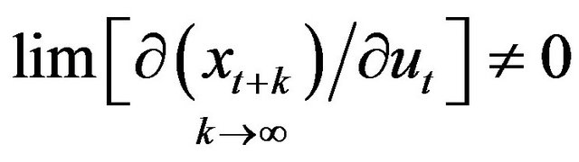
It implies that money should be non-stationary in level .
.
Fisher and Seater (1993) show that for ,
,  can be written as,
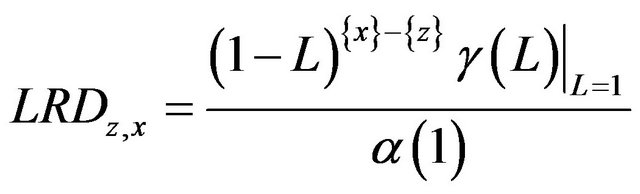 (3)
(3)
where 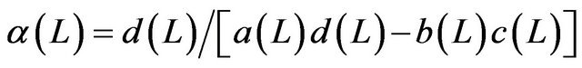
and 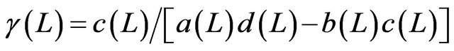
It is seen that the long run derivative of z with respect to x depends on .
.
2.2. Identification
The identification problem is dealt with by imposing the exogeneity of money in the long run by assuming . After this assumption, Fisher and Seater (1993) establish that
  equals to the frequency zero regression coefficient when
  is regressed on
 . The estimator of
  is obtained by
 ,
,  is the slope coefficient of the following regression,
 (4)
(4)
The appropriate models for the following special cases:
1) When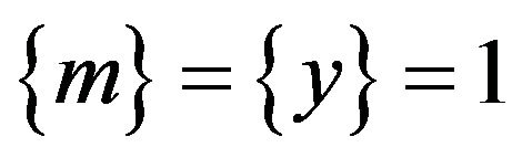 , the LMN is tested by applying Equation (5) to estimate
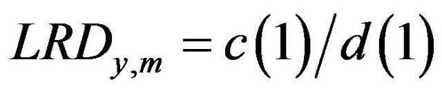 ,
,
 (5)
(5)
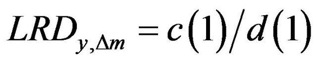
2) When  and
and , LMN cannot be rejected and LMSN can be tested by deriving the following equation to estimate,
 (6)
(6)
3) When , in this case
which means that permanent change in the growth rate of money affects the growth rate of output in the same way the level of money affects the level of output. Therefore, this implies that “growth-rate to growth-rate” propositions are not LMSN propositions. To test LMSN in this case, first of all LMN should be held. If LMN holds, then LMSN can be tested by deriving Equation (8) to estimate,
Thus LMN: 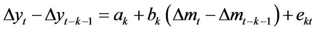 (7)
(7)
LMSN: 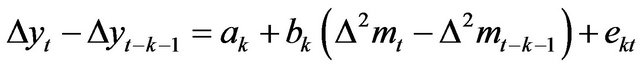 (8)
(8)
These linear Equations (5)-(8) can be computed by applying Newey and West (1987) [10] approach to obtain consistent estimate of . These authors purpose a consistent covariance matrix estimator by applying GMM methodology when error terms are heteroskedastic and autocorrelated.
3. Data
As indicated in Leong and McAleer (2000), the result of LMN test is sensitive to underlying monetary aggregate. We cannot claim LMN only depending on one money aggregate. Therefore, we consider all alternative monetary aggregates: M1, M2 and domestic credit in EMCCA namely, Cameroon, Central African Republic, Chad, Congo Brazzaville and Gabon. Guinea Equatorial was not considered because of data availability. As a real output measure, GDP series at fixed 2000 prices is considered. The CPI with 2000 base year is used to obtain an inflation series. All of the variables are obtained from the Word Bank Data set, the World Development Indicators, covering the periods 1970-2008. They are obtained on yearly basis.
The contemporary economic history of EMCCA countries can be summarized in four main eras: 1960-1980, strong economic expansion; 1981-1994, economic and financial crises, then devaluation of the local currency in 1994; 1995-2005, implementation of stabilization programs with mitigating results; 2005 onward economic stability and growth era. During the 1960-2010 period the average inflation was 5% and the real GDP growth rate was on average 3.5% with 2.5% percent volatility. However, during 1981-1993 period, inflation decreased to one digit, and real GDP growth on average increased to 4.2%, with 4.5% volatility. In EMCCA, from 1970 to 1995 there was high and persistent inflation and unstable economic growth. The 1993 crisis has been followed by the 1994 devaluation of the domestic currency. The inflation reached to 12%. In 1999 financial crisis occurred as an infection of world financial crises and in 2001 the deepest financial melt down took place. However, after 2002 based on IMF and the World Bank stabilization programs, monetary stability has been employed as a framework for monetary policy. Inflation decreased to one digit. The low level inflation has been accompanied by a significant decrease in money supply growth. Indeed, stable economic growth has been achieved. Thus, during the 1960-2010 period EMCCA faced with challenging economic events, economic and financial crises. There were sudden changes in money and prices. Therefore, although our period is relatively shorter, this data set is qualified to be used for controlling a long run relationship.
In this study, we use real GDP and all monetary aggregates in their logarithms. Since all the series are annually, there is no need to test for seasonality.
4. Econometric Results
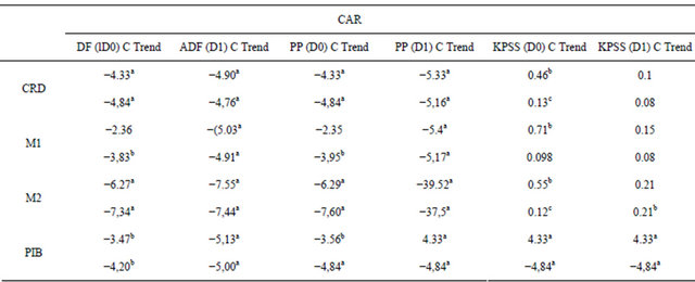
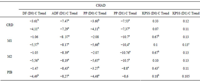
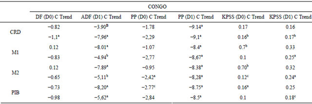
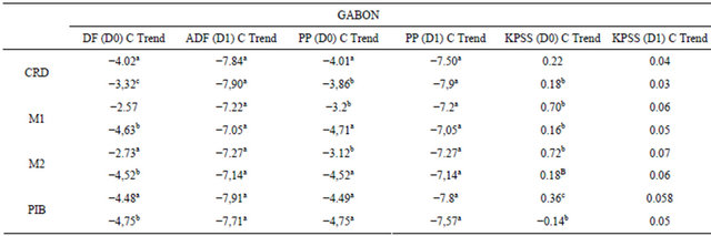
In the Fisher and Seater (1993) methodology, the nonstationarity of the variables (money aggregates and real output) is the necessary condition to test LMN. Therefore, the Augmented Dickey-Fuller (1979) (ADF), Phillips and Perron (1988) (PP), and Kwiatkowski et al. (1992) (KPSS) unit root tests are applied to the series involved [11-13]. The results of the above tests suggest that all of the variables are I(1) for all the countries considered in this analysis.
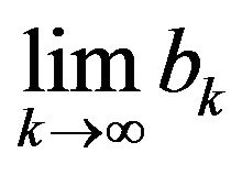
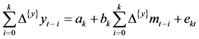
The Fisher and Seater (1993) analysis provides a straightforward test of LMN. Since real GDP and money aggregates are I(1), the long run derivative of real GDP with respect to money is equal to the slope coefficient of a regression of growth rates of real GDP on growth rates of money. Thus, the LMN hypothesis will be examined by using Equation (5). LMN is sustained if the slope coefficient  goes to zero as
  goes to infinity.
Confidence intervals around estimated  respectively are determined for M1, M2 and domestic credit. The estimates of
  are obtained for
 . The 95 percent confidence intervals are constructed for the estimated coefficient of money supply using t-distribution with
  degrees of freedom. The standard errors employed to construct the confidence intervals are corrected for autocorrelation and heteroskedasticity by the Newey and West (1987) method. As an example, we present in Figure 1, the graphs of confidence intervals for bk in the case of Cameroon (country leader) and Gabon (EMCCA second economy).
The econometric results obtained can be summarized as follows:
1) For all, using M1, M2 and domestic credit, we could not find evidence in favor of the LMN hypothesis; in fact, the tests consistently reject the LMN hypothesis;
2) All the estimates of  are significant and positive for all countries;
3) As a result there is a significant and positive effect of M1, M2 and domestic credit on real GDP in the long run.
In order to cross-check the above results, the same estimations were conducted on different sub-periods and the new estimates of  were obtained. Again, the results indicate strong support in favor of the positive impacts of money aggregates on real GDP.
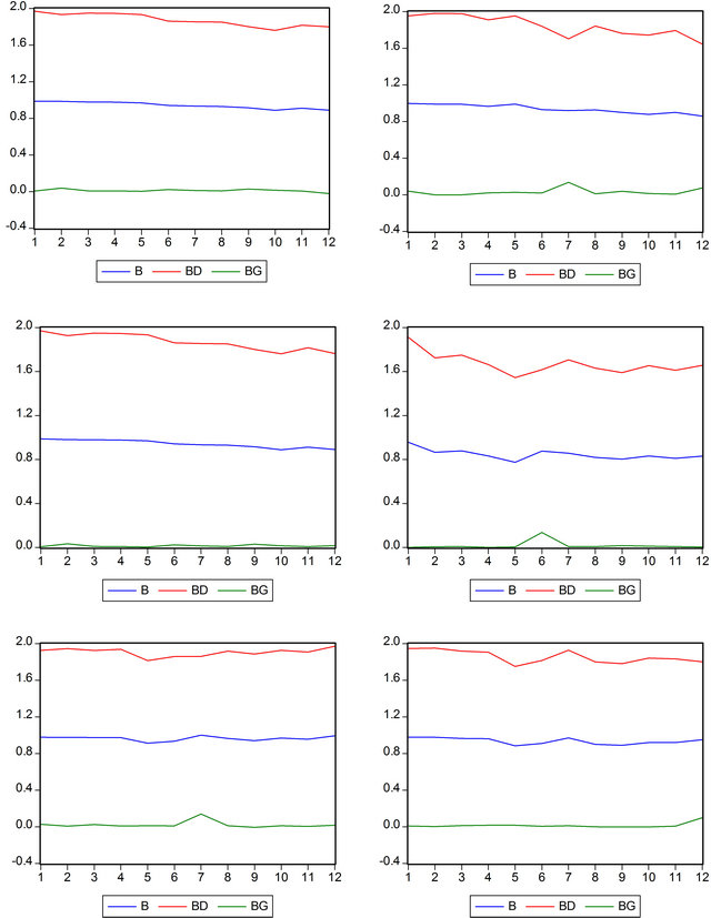
Figure 1. Graphs of confidence intervals for the credit, M1 and M2 in the case of Cameroon (left) and Gabon (right).
Finally, Chow tests were used to check the stability of the estimates of . The breakpoints used were 1991 period of major banking reforms in EMCCA and 1994 period of devaluation of the local currency. The breakpoints were used separately and then jointly in the analyses. Results which are available upon requests from the author strongly support the findings that the estimates of
  are stable and also that the previous results are not altered in any cases. Thus, confirming the significant and positive impacts of money aggregates on real GDP in EMCCA.
5. Final Remarks
This paper has analyzed the LMN hypothesis in the case of EMCCA. Econometric results indicate consistently and significantly that money aggregates have positive impacts on real GDP in the long run. That means the LMN hypothesis is rejected.
The implication of this result is that in the context of poverty and unemployment that characterizes EMCCA countries, the Central Bank should pursue an objective of stabilization of the product, along with the objective of monetary stability.
Finally, it would be desirable to see if the results are confirmed in the context of the VAR methodology proposed by King and Watson (1997).
REFERENCES
- M. E. Fisher and J. J. Seater, “Long Run Neutrality and Super Neutrality in an ARIMA Framework,” American Economic Review, Vol. 83, No. 3, 1993, pp. 402-415.
- R. G. King and M. W. Watson, “Testing Long Run Neutrality,” Federal Reserve Bank of Richmond Economic Quarterly, Vol. 83, No. 3, 1997, pp. 69-101.
- A. A. Weber, “Testing Long Run Neutrality: Empirical Evidence for G7 Countries with Special Emphasis on Germany,” Carnegie-Rochester Conference Series on Public Policy, Vol. 41, No. 1, 1994, pp. 67-117.
- N. Serletis and Z. Koustas, “International Evidence on the Neutrality of Money,” Journal of Money, Credit and Banking, Vol. 30, No. 1, 1998, pp. 1-25.
- K. Leong and M. McAleer, “Testing Long Run Neutrality Using Intra-Year Data,” Applied Economics, Vol. 32, No. 4, 2000, pp. 25-37.
- G. L. Shelley and F. H. Wallace, “Long Run Effects of Money on Real Consumption and Investment in the US,” International Journal of Applied Economics, Vol. 3, No. 1, 2006, pp. 71-88.
- S. K. Bae and R. A. Ratti, “Long Run Neutrality, High Inflation and Bank Insolvencies in Argentina and Brazil,” Journal of Monetary Economics, Vol. 46, No. 3, 2000, pp. 581-604.
- S. N. Sulku, “Testing the Long Run Neutrality of Money in a Developing Country: Evidence from Turkey,” Journal of Applied Economics and Business Research, Vol. 1, No. 2, 2011, pp. 65-74.
- S. W. Chen, “Evidence of the Long Run Neutrality of Money: The Case of South Korea and Chinese Taiwan,” Economics Bulletin, Vol. 3, No. 2, 2007, pp. 1-18.
- W. K. Newey and K. D. West, “A Simple, Positive SemiDefinite, Heteroskedasticity and Autocorrelation Consistent Covariance Matrix,” Econometrica, Vol. 55, No. 3, 1987, pp. 703-708.
- D. A. Dickey and W. A. Fuller, “Likelihood Ratio Test Statistics for Autoregressive Time Series with a Unit Root,” Econometrica, Vol. 49, No. 1, 1981, pp. 1057-1072.
- P. C. B. Phillips and P. Perron, “Testing for a Unit Root in Time Series Regressions,” Biometrika, Vol. 75, 1998, pp. 335-346.
- D. Kwiatkowski, P. C. B. Phillips, P. Schmidt and Y. Shin, “Testing the Null Hypothesis of Stationarity against the Alternative of a Unit Root: How Sure Are We that Economic Series Have a Unit Root,” Journal of Econometrics, Vol. 54, No. 1, 1992, pp. 159-178.
Appendix: Unit Root Tests

Notes: a, b and c indicate statistical significance at 1, 5 and 10 percent level respectively.
Notes: a, b and c indicate statistical significance at 1, 5 and 10 percent level respectively.
Notes: a, b and c indicate statistical significance at 1, 5 and 10 percent level respectively.
Notes: a, b and c indicate statistical significance at 1, 5 and 10 percent level respectively.
Notes: a, b and c indicate statistical significance at 1, 5 and 10 percent level respectively.