ABSTRACT

Normal trade in goods assumes two sectors that co-exist for reasons such as comparative advantage and interact via trade. Arbitrage trade in goods assumes two markets that artificially exist and converge via trade. Restoration of the law of one price via arbitrage creates one sector out of two, and in general equilibrium, equalizes opportunity cost of resources used in production. Arbitrage does not occur in a vacuum, such that when the high (low) price of a good decreases (increases) in its artificially segmented market during arbitrage, the supply of the good falls (rises), the resources used intensively in that good earn lower (higher) returns, affecting security prices, and the supply of those resources in that good’s production fall (rise).

1. Introduction

Arbitrage, possible when a good has different prices in multiple markets, can restore the “law of one price”. In contrast to normal trade, with markets that co-exist for reasons like comparative advantage and interact via trade, arbitrage leads to convergence via trade of markets that artificially exist. Restoration of the law of one price via arbitrage creates one sector out of two, and in general equilibrium, equalizes opportunity cost of resources used in production. How arbitrage in goods interacts with securities (and more broadly resources) is left unanswered, as arbitrage is usually examined in partial equilibrium. This paper examines goods arbitrage in general equilibrium, with arbitrage caused movement of goods prices interacting and affecting resource prices—capital (securities) and labor.

In the literature, the classic work on general equilibrium arbitrage by Harrison and Kreps [1] applies only to securities. Werner [2] considers a general equilibrium model of markets that include both commodities and assets, and shows that no arbitrage opportunities are sufficient for general equilibrium. Dana, Le Van and Magnien [3] give conditions for the absence of arbitrage and existence of equilibrium, including an extensive literature review. Page, Wooders and Monteiro [4] also show that inconsequential arbitrage—arbitrarily large arbitrage opportunities—is sufficient for equilibrium. And Kuksin [5]

examines the relationship between the efficient market hypotheses and general equilibrium, where economic inefficiency leads to market inefficiency as it reduces the information necessary for efficient prices.

This paper fits within the literature that combines efficient pricing of securities and absence of arbitrage in finance with competitive equilibrium in economics. In examining arbitrage in general equilibrium, it describes the processes that arbitrage in goods has on the pricing of capital (securities) and labor, and the effects that this has on resources and goods. A key aspect is that arbitrage does not occur in a vacuum, but has real effects on resources and goods, as it reverses the process of normal trade by combining two artificial sectors into one, affecting rewards to and supply of resources, and supply of outputs as formerly divided sectors unite.

Purchasing power parity (Cassel [6] and Roll [7]), capital structure theory (Modigliani and Miller [8] and Modigliani and Miller [9]) and arbitrage pricing theory (Ross [10] and Roll and Ross [11]) use arbitrage in partial equilibrium, insofar as there is an absence of the effects of arbitrage on other agents. A general equilibrium approach would fill this void, such as Varela and Olson [12] in their investigation of the factor returns and output effects on a regulated and unregulated sector from imposition of a rate of return on investment regulatory constraint, and Varela [13] in using a general equilibrium framework to complete the Modigliani‑Miller capital structure arbitrage propositions.

Section 2 presents the general framework in which the arbitrage process occurs and previews the overall results. Section 3 presents the model used to analyze this framework and derive its basic conclusions. Section 4 provides the implications of the general equilibrium model for arbitrage. Section 5 presents an overall summary.

2. The Framework and Preview of Results

The arbitrager is a trader, serving as an intermediary between two markets for the same good. Each market is serviced by representative firms selling the “same” product for different prices. These firms can be theoretically constructed, as the conditions for a firm to exist are present whether or not it does, because trading in the absence of a firm can substitute for the existence of a firm. That is, a firm producing in market “i” and selling in market “j” (presumably for the higher price) is equivalent to a firm producing and selling in market “j” for the higher price, as the former’s firm’s resources are rewarded based on market “j’s” price. The general equilibrium effects of arbitrage concern how the arbitrager’s trading activity as an intermediary between our two markets affects the economic positions of our two theoretically constructed and representative firms.1 The framework requires that two representative firms, or classes of firms, exist in a general equilibrium model, based on Jones [14] methodology.2 The firms employ capital and labor to produce the same product in different markets at different prices, with these markets segmented for these firms.3 An arbitrager is introduced who can circumvent the market segmentation, arbitrage the goods’ price differences, and affect the prices in each market. The general equilibrium approach examines these effects from arbitrage on our representative firms, or classes of firms, with respect to output, employment and rewards to resources. The fact that the arbitrager’s activity will be shown to have an effect on these variables justifies a general equilibrium view of arbitrage.

The arbitrage will cause the price of the good in the low (high) price market to rise (fall), with associated effects on the representative firms in each market. All else the same, the increase (decrease) in the low (high) price will produce increases (decreases) in the supply of the low (high) priced good, increases (decreases) in the reward to the resource used intensively in the production of that good, and increases (decreases) in the amount of resources used in the production of that good.

The effect of the arbitrage on product price will impact income distributions between resources used in a product’s production and the way in which they are employed, both within and between the two sectors. Clearly, arbitrage does not occur in a vacuum and has real effects, whether on existing firms in each sector, or on theoretically constructed firms, such that the influences of arbitrage also affect potential new entrants in the markets.

3. The Model

3.1. Foundation

A good that should competitively have the same price instead trades in two markets for different prices, making arbitrage feasible. This situation is modeled using Jones’ [14] two sector model, with its competitive conditions modified because the assumed price differences between markets make the initial equilibrium conditions local instead of global.

A good exists that while physically the same has different prices in different markets, identified as good B when it bears a big price, P_B, in market B, and good S when it bears a small price, P_S, in market S. This good in markets B and S is produced using labor and capital, with total available labor supply L and capital supply K. Technically implied in their prices is that B uses more of the more expensive resource (we assume labor) in production compared to S which uses more of the less expensive resource (we assume capital). The higher opportunity cost for producing (supplying) B explains the higher price for B, and lower opportunity cost for producing S accounts for the lower price for S, under local competitive conditions.

The effects of arbitrage on good prices affects resource prices in general equilibrium, even if a firm and production in a market does not exist, because the prices in question affect potential entrants to these markets and the opportunity costs of resources in these markets. The higher price for B implicitly reflects higher opportunity costs in market B; the lower price for S implicitly reflects lower opportunity costs in market S. The absence of a global equilibrium price for the good implies lack of a global equilibrium opportunity cost in its production. It also simultaneously motivates the arbitrage, for arbitragers are indifferent to the cause of the price differences or opportunity costs, so long as the good can be traded to their advantage, until the markets converge.

3.2. Conditions

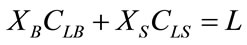
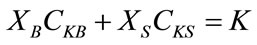
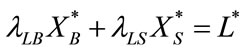
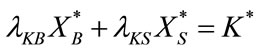
Total production of B and S equals X_B and X_S. The labor and capital used per unit of good B is C_LB and C_KB, and per unit of S is C_LS and C_KS. The labor to capital ratio in good B is higher than in S.4 All available labor L and capital K are employed, such that

(1a)

(1b)

where labor and capital used in production is L_B and K_B for B, and L_S and K_S for S, and C_LB = L_B/X_B, C_LS = L_S/X_S, C_KB = K_B/X_B; and C_KS = K_S/X_S.

The cost of labor (wage rate per unit of labor or required return to labor) is k_Li and the cost of the capital (interest rate or required return to capital) is k_Ki for firms in sector i, i = B, S.

Competitive global resource conditions equalize the respective returns to labor and capital in both sectors, such that k_LB = k_LS = k_L, and k_KB = k_KS = k_K.

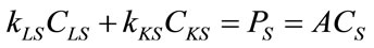
Competitive local goods conditions in each sector (although not between sectors) requires that the price in each sector equal its respective long run average cost, such that

(2a)

(2b)

where P_i equals the final product price and AC_i equals the average cost of production respectively for firms in sector i, i = B, S.

The arbitrager buys at the low price (P_S) and sells at the high price (P_B), leading to a decrease in P_B and increase in P_S. The effect of these changes in prices on our representative firm or group of firms—that is the general equilibrium effects of arbitrage—is examined next.

3.3. Dynamics with Respect to Factor Supplies and Output

The equations of change in outputs from total differentiation of (1a) and (1b) show the effects of changes in L and K on X_B and X_S, such that (with algebraic manipulations)⁵

(3a)

(3b)

where λ_LB = L_B/L; λ_LS = L_S/L; λ_KB = K_B/K; λ_KS = K_S/K; L^* = dL/L; K^* = dK/K; = dX_B/X_B; and = dX_S/X_S.

Solving the system (3) for and, obtain

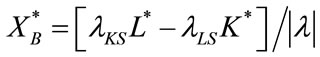(4a)

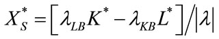(4b)

where describes factor intensities in the physical sense, such that

(5)

and c/l_S and c/l_B are the physical capital to labor ratios for firms in sectors S and B.

The result in (4) is the well-known Rybczynski [16] theorem. Assume that sector B is labor and S is capital intense in the physical sense, i.e.. If the capital supply is constant (K^* = 0) and the labor supply increases (L^* > 0), then in (4a) is positive (the output of the labor intense sector B rises) and in (4b) is negative (the output of the capital intense sector S falls). If the capital supply increases (K^* > 0) and the labor supply is constant (L^* = 0), then is negative and is positive. Opposite results hold when. Subsequently, in this paper, Rybczynski’s theorem is used in reverse as arbitrage merges two sectors into one.

3.4. Dynamics with Respect to Final Product Prices and Factor Rewards

The equations of change in prices from total differentiation of (2a) and (2b) show the effects of a change in prices P_B and P_S on factor rewards k_L and k_K, such that (with algebraic manipulations)6

(6a)

(6b)

where θ_LB = k_LL_B/P_BX_B; θ_LS = k_LL_S/P_SX_S; θ_KB = k_KK_B/P_BX_B; θ_KS = k_KK_S/P_SX_S; = dP_B/P_B; = dP_S/P_S; = dk_L/k_L; and = dk_K/k_K.

Solving the system (6) for and, obtain

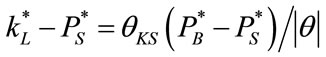(7a)

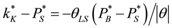(7b)

where describes factor intensities in the value sense, such that

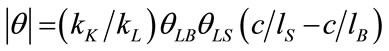(8)

The result in (7) is the well-known Stolper and Samuelson [17] theorem. Assume that sector B is labor intense and S is capital intense in the value sense, i.e.. If the price of B increases (> 0) and of S is constant (= 0), then in (7a) is positive and in (7b) is negative. If the price of B is constant (= 0) and of S increases (> 0), then in (7a) is negative and in (7b) is positive. The rewards to resources used intensively (unintensively) in production of a good are positively (negatively) correlated with the change in the price of that good. Opposite results exist when. Subsequently, in this paper, Stolper-Samuelson’s theorem is used in reverse as arbitrage merges two sectors into one.

3.5. Dynamics with Respect to Prices and Output

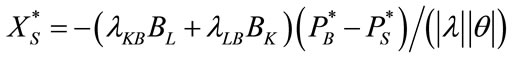
Interaction between the equations of change in prices and outputs, given the elasticity of substitution and minimum cost conditions in each sector, shows the effects of a change in final product prices on final product outputs, such that

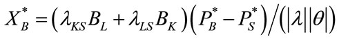(9a)

(9b)

where B_L = (λ_LBθ_KBσ_B + λ_LSθ_KSσ_S)/|θ|, and B_K = (λ_KBθ_LBσ_B + λ_KSθ_LSσ_S)/|θ|, where the elasticities of substitution in each sector, σ_B and σ_S, are positive as σ_i = (–)/( –), i = B, S, and the numerators of B_L and B_S are positive.

Since the sign of is directly and is inversely related to the sign of (–), as without distortions—no factor intensity reversals—both and have the same sign such that their product is positive, it follows that normal upward sloping supply functions exist.

3.6. Summary

Under conditions of general equilibrium, firms in an economy will produce more (less) of a good that uses in production its most (least) relatively abundant factor, reward more (less) the factor that is used most (least) in the production of a product when that product’s price rises, and operate with normal supply functions in the absence of factor intensity reversals.

4. General Equilibrium Implications of Arbitrage

Two markets are defined by their prices for the same good, with one high priced B and the other low priced S, with actual or theoretically (potentially) constructed firms in each. The good may be produced in both markets, although this is not absolutely necessary, for trading in the absence of production is a substitute for production. Markets B and S do not exist because of fundamentals such as comparative advantage, but because they are artificially segmented. The arbitrager is allowed to be the intermediary trader, buying low and selling high, integrating these artificially segmented markets which converge into one. The arbitrage process causes S’s price to rise and B’s to fall, with associated general equilibrium effects on real and financial variables in each. As these effects involve a reversal in the normal process that creates two markets or sectors in an economy, the normal theorems in the two-sector model operate in reverse to obtain the general equilibrium effects as markets unify.  

Under normal conditions, with no factor intensity reversals, supply functions are normal, such that as shown in (9a) and (9b), arbitrage driven price increases in market S (> 0) cause the output of good S to rise (> 0), and price decreases in B (< 0) cause the output of B to fall (< 0). The Stolper-Samuelson theorem from (7a) and (7b) then shows that as the price of S rises (> 0), the resource used intensively in its production (which depends on the sign of) earns higher returns while the other resource earns lower returns.

As S is assumed to use capital intensively in a value sense (> 0), the return to capital in S rises (> 0) and the return to labor in S falls (< 0). Similarly, as the price of B falls (< 0), the resource used intensively in its production earns a lower return while the other resource earns a higher return. As B is assumed to use labor intensively in a value sense (> 0), the return to labor in B falls (< 0) and the return to capital in B rises (> 0). Since capital is financed by the sale of securities, the increase in the return to capital in both B and S reduces security prices as goods arbitrage occurs, so long as market S is capital and B is labor intense in a value sense. Security prices would rise if market S was labor and B was capital intense in a value sense.

Overall, when the high priced good is labor intense and rewards labor more than it should, and the low priced is capital intense and rewards capital less than it should, i.e. the relative cost of labor is higher than required, market convergence from arbitrage causes the return to capital to rise, security prices to fall, and the return to labor to fall throughout. When arbitrage in a good results in equilibrium in the good’s price in line with the law of one price, the general equilibrium effects on resources are such that the relative costs of resources also achieve equilibrium.

Further, the Rybczynski theorem from (4a) and (4b) shows that as production of good S rises (> 0), a greater supply of capital (K^* > 0) is needed in S to engage in its production, and as production of B falls (< 0), a lower supply of labor (L^* < 0) is needed in B. These effects will be applicable to firms that produce or enter the market to produce B or S. An arbitrager exploiting mispricing in markets causes real effects on output supplies, as well as the amounts of resources utilized in each market, and their real rewards. More resources will be used in the low priced market as its product price rises, and the resources used intensively therein will earn higher rewards. Fewer resources will be used in the high priced market as its product price falls, and the resources used intensively therein will earn lower rewards. The arbitrager who affects product prices in each sector does not operate in a partial equilibrium vacuum.

5. Summary and Conclusions

Normal trade theory assumes two sectors that naturally co-exist, for reasons such as comparative advantage, and interact via trade. Arbitrage assumes two markets that artificially co-exist, with the arbitrager serving as the agent that causes the markets to interact via trade that exploits their artificial mispricing. Arbitrage unites these two artificially created markets as they merge into one. Most discussion of the arbitrage process examines how it ultimately satisfies the law of one price, without much elaboration on the real effects associated with the associated changes in prices. This paper fills this void, showing the real effects on output, resource utilization and resource rewards associated with the arbitrage process in goods.

Arbitragers are keen in noticing violations of the law of one price. They buy a good in one market for a low price and sell it in another for a high price, and earn arbitrage profits. This activity does not occur in a vacuum. What happens to other agents (or theoretically constructed agents) in the market, and firms, as the arbitrage process restores the law of one price? This paper uses well known propositions in two sectors general equilibrium models in reverse when applied to the arbitrage process, because arbitrage reverses a product’s presence in two markets—the high and low priced markets—as two sectors converge into one.

A product where the law of one price is violated exists in two markets. The market forces from the arbitrage process decrease the high product price and increase the low product price. As the high price decreases, the supply of the product falls in that market, the resources used intensively in that product earn lower returns and the supply of those resources in that product’s production fall. As the low price increases, the supply of the product rises in that market, the resources used intensively in that product earn higher returns and the supply of those resources in that product’s production rise. The firms— theoretically constructed or potential new entrants—operating in each market merge in an operational sense when one price is restored. These firms then have similar capital to labor ratios, the product has the same price, the rewards to the resources are consistent with the law of one price, and the product output is driven by one price.

REFERENCES

NOTES

^*Varela thanks the College of Business Administration at the University of Texas at El Paso for summer 2009 research support for this work. Any errors in this research are the sole responsibility of the author.

¹We only allow the arbitrager to intermediate between markets, and not the firms, in order to maintain purity in the analysis between the arbitrage activity and its economic effects, although both of these could be incorporated into one if the firm was also an arbitrager.

²An excellent application of this model in international trade is in Batra, [15].

³The general equilibrium model is general in the sense that not only can final product prices that are subject to arbitrage be analyzed, but resource prices such as labor and capital that are subject to arbitrage can also be analyzed. In this paper, we only concentrate on final product prices, although resource prices provide some basis for extensions in this research. The final product prices may initially be different in each market owing to some restriction, such as capital, trading or informational restrictions, or exchange rate controls, that the arbitrager is able to circumvent.

⁴The fundamental results are not changed if the ratio of labor to capital in good B is lower. One reason that the ratio of labor to capital in each market is different is that the final product price in each market is different. As in this case the value of the outputs are different in each market, the ratio of the value of labor and capital to output will also be different in each. Another reason is that resources are misallocated, such that more of the more expensive resource is used in the high price market.

⁵In this part of the analysis, final product prices are assumed constant, and therefore so are each sector’s input-output coefficients, such that, , and equal zero. Note: = dC_LB/C_LB; = dC_LS/C_LS; = dC_KB/C_KB; and = dC_KS/C_KS.

⁶Recall that for the cost of labor, k_LB = k_LS = k_L, and for the cost of capital, k_KB = k_KS = k_K. Also, in this analysis, long‑run profit maximization with pure competition in each sector requires that the firm’s perfectly elastic demand curve (marginal revenue) equal its marginal cost, a condition satisfied at the minimum point on the firm’s average cost function. Therefore, the terms associated with this condition in (6a) and (6b) vanish, that is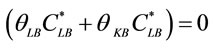, and

REFERENCES

- J. M. Harrison and D. M. Kreps, “Martingales and Arbitrage in Multiperiod Securities Markets,” Journal of Economic Theory, Vol. 20, No. 3, 1979, pp. 381-408. doi:10.1016/0022-0531(79)90043-7
- J. Werner, “Arbitrage and the Existence of Competitive Equilibrium,” Econometrica, Vol. 55, No. 6, 1987, pp. 1403-1418. doi:10.2307/1913563
- R. A. Dana, C. Le Van and F. Magnien, “On the Different Notions of Arbitrage and Existence of Equilibrium,” Journal of Economic Theory, Vol. 87, No. 1, 1999, pp. 169-193. doi:10.1006/jeth.1999.2518
- F. H. Page Jr., M. H. Wooders and P. K. Monteiro, “Inconsequential Arbitrage,” Journal of Mathematical Economics, Vol. 34, Vol. 4, 2000, pp. 439-469.
- N. Kuksin, “General Equilibrium: Arbitrage and Information,” Centre for Economic Reform and Transformation Discussion Paper No. 701, Heriot Watt University, Edinburgh, 2007.
- G. Cassel, “The World’s Monetary Problems,” Constable and Company, London, 1921.
- R. Roll, “Violations of Purchasing Power Parity and Their Implications for Efficient International Commodity Markets,” In: M. Sarnat and G. Szego, Eds., International Finance and Trade, Vol. 1, Ballinger Pub. Co., Cambridge, 1979, pp. 133-176.
- F. Modigliani and M. H. Miller, “The Cost of Capital, Corporation Finance and the Theory of Investment,” American Economic Review, Vol. 48, No. 3, l958, pp. 26l-297.
- F. Modigliani and M. H. Miller, “The Cost of Capital, Corporation Finance and the Theory of Investment: Reply,” American Economic Review, Vol. 49, No. 4, 1959, pp. 655‑667.
- S. A. Ross, “The Arbitrage Theory of Capital Asset Pricing,” Journal of Economic Theory, Vol. 13, No. 3, 1976, pp. 341-360. doi:10.1016/0022-0531(76)90046-6
- R. Roll and S. A. Ross, “An Empirical Investigation of the Arbitrage Pricing Theory,” Journal of Finance, Vol. 35, No. 5, 1980, pp. 1073-1103.
- O. Varela and R. E. Olson, “A General Equilibrium Analysis of Financial Regulation,” Journal of Public Economics, Vol. 30, No. 3, 1986, pp. 329-340. doi:10.1016/0047-2727(86)90054-X
- O. Varela, “Firms’ Factor Cost Responses to the Modigliani-Miller Propositions,” Review of Business and Economic Research, Vol. 22, No. 1, 1986, pp. 55-68.
- R. W. Jones, “The Structure of Simple General Equilibrium Models,” Journal of Political Economy, Vol. 73, No. 6, 1965, pp. 557-572.
- R. N. Batra, “Studies in the Pure Theory of International Trade,” St. Martin’s Press, New York, 1973.
- T. B. Rybczynski, “Factor Endowment and Relative Commodity Prices,” Economica, Vol. 22, No. 88, 1955, pp. 336-341. doi:10.2307/2551188
- W. Stolper and P. Samuelson, “Protection and Real Wages,” Review of Economic Studies, Vol. 9, No. 1, 1941, pp. 58-73. doi:10.2307/2967638