Modern Economy
Vol.3 No.2(2012), Article ID:18135,8 pages DOI:10.4236/me.2012.32024
Pricing for Basket CDS and LCDS
Department of Mathematics, Tongji University, Shanghai, China
Email: liang_jin@tongji.edu.cn
Received December 14, 2011; revised January 29, 2012; accepted February 11, 2012
Keywords: Basket Loan-Only Credit Default Swap; Prepayment Risk; Bottom Up; Reduced Form; One Factor ICIR Model
ABSTRACT
In this paper, under the reduced form framework and “Bottom Up” method, a model for pricing a basket Loan-only Credit Default Swap (LCDS), with the negative correlation between prepayment and default, is established. A general pricing formula for it is obtained, where one factor CIR (Cox-Ingersoll-Ross) and ICIR (Inversed CIR) models are used to describe the negative correlation between prepayment and default. In this situation, the positivity of prepayment and default intensity processes are guaranteed. Numerical computations are presented.
1. Introduction
During the last twenty years, the market for credit derivatives has experienced rapid development with the increasingly prominent importance of derivatives which leads to the evolution and innovation of the credit market.
The international financial crisis began in the year 2008 shocked the financial market even the global economy. Since assets securitization contributed a lot to the financial crisis, recent researches focus more and more on measuring the related risks and prices. Academic studies usually analyze the risks of interest rate, prepayment, default etc., which are related to the asset securitization products by building mathematical models. Then they try to use methods of stochastic processes, partial differential equations and statistics etc. to obtain solutions analytically, or use finite differential methods and the Monte Carlo simulation etc. to study empirical data and solution numerically.
The two classical frameworks in the mathematical modeling of the problem are the structural and reducedform methods. Among them, the reduced-form method has peerless advantages than the structural method in pricing credit derivatives with large asset pools. Then as a result, many new methods and techniques have been developed within the reduced-form framework in recent years, especially for pricing basket CDS, CDO and LCDS etc. The reduced-form method can be divided into two categories: “Bottom Up” ([1,2]) and “Top Down” ([3,4]) frameworks. In the first one, the events probability distributions of the whole asset pool are obtained after the intensity models of every reference contract being built. Nevertheless, in the second one, the model focuses on the whole asset pool, and the parameters of the model can be estimated from statistical data. Once the events are modeled, the pricing formula can be obtained by using PDEs or statistical methods. Furthermore, numerical methods such as finite differentiation can be applied for numerical analysis.
We begin pricing basket CDS, which helps us better understand the pricing model of basket LCDS. Under the assumption that the default intensity follows a Vasicek model, Junmei Ma and Jin Liang ([5]) obtained the joint survive probability distribution function of N assets with PDEs. Tao Wang and Jin Liang ([6]) employed Monte Carlo method to verify the above model and analyzed its effective range. In more details, Jin Liang et al. ([7]) pointed out that the Vasicek model is accurate only when the asset pool is a small one, and it does not fit the reality when the scale of the asset pool increases to some extent. Therefore, it is reasonable that the positive default intensity should be guaranteed by replacing the Vasicek model with a CIR model, though the correlation between different assets increase the dimension of the PDE and bring more difficulties in solving this problem.
Loan Credit Default Swaps (LCDS) are almost identical to the standard Credit Default Swaps (CDS) except two features. 1) The reference obligation of a LCDS contract is limited on loans; 2) LCDS contract can be cancelled. This means that correlated prepayment and default should be both considered. Therefore, pricing a LCDS is not simply extending from pricing a standard CDS. The situation for basket LCDS makes problem more complicated. Literatures on pricing a single-name LCDS include ex. Wei ([8]) and Liang & Wang ([9]). By use of “top down” framework, pricing a basket LCDS is considered in Liang and Zhou ([10,11]) and Wu and Liang ([12]).
In this article, the Bottom Up method is used to price basket CDS and LCDS. We use a factor model to describe the correlation of the prepayment and default among the references. This model is developed step by step from Pricing a basket CDS, the simplest basket LCDS (two references) to large-scale basket LCDS to obtain the formulae.
The structure of the paper as follows: In the next Section 2, a model of pricing basket CDS with CIR process is discussed. In Section 3, a simplest basket LCDS, which includes two loan references, is considered. Then the model is extended to a large scale of basket LCDS in Section 4. Numerical examples are shown in Section 5. Section 6 is conclusion.
2. Basket CDS Pricing with CIR Intensities
According to [5], the basket CDS can be priced given the joint survive probability of reference assets (here we assume the assets are all residential mortgage loans) in the pool. If the prepayment is neglected, this CDS is a special case of a basket LCDS. In the following paragraphs the single factor CIR model will be used to build to the dependency of the reference loans.
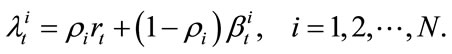
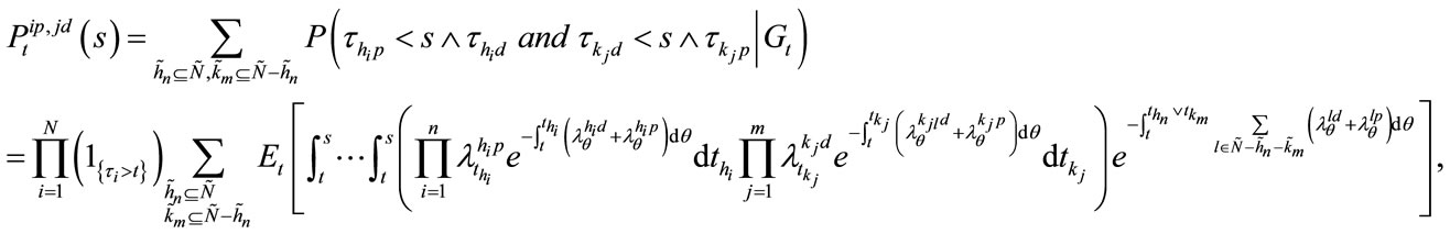
We assume that the number of reference loans in the pool is , and describe the default process of every loan with non-homogenous Poisson process. The default intensities
 satisfy the following single factor models:
 (1)
(1)
in which  are correlation coefficients, and
  and
and  are drove by CIR processes.
Denote  as the default times of loan
 .
.  are stopping times defined in a probability space
 , where
  represents the information flow formed by all the information in the market, and
 is the risk-neutral probability measure,
 and
and  includes all the known information in the market.
is the default indicating process of loan ,
, 
According to the definition of reduced form method, the unity survive probability from time  to time
 ![]() is
is
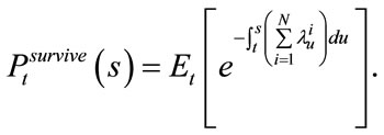 (2)
(2)
According to the solving method in [9,12], one can obtain
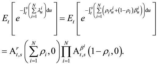 (3)
(3)
where
 (4)
(4)
 (5)
(5)
And thus the explicit expression for the joint survive probability 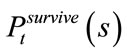 can be obtained, which is shown in Figure 1.
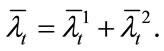
Figure 2 is a price picture of large scale nth-to-default basket CDS, and the coefficients are the same as [6]. The picture indicates that the pricing formula still corresponds to reality when the asset amount exceeds that in [6]. Thus the CIR model fills the gap in the model using Vasicek process. The model can be applied to evaluate larger-scale basket CDS than those shown in the figure, and it is more proficient. Estimating from the current calculation efficiency, it takes about 10 to 20 minutes to price an nth-to-default basket CDS with 120 loans.
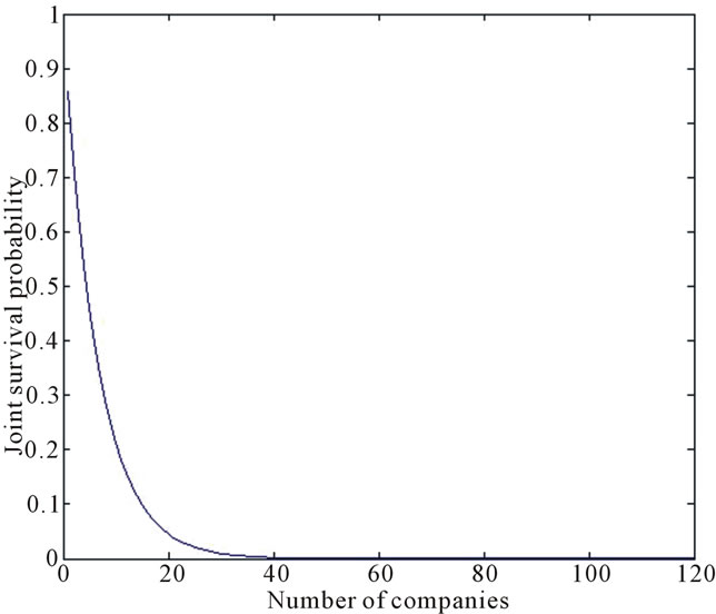
Figure 1. Joint survival probability.
Figure 2. Fair price of basket nth-to-default CDS.
3. Pricing the Simplest Basket LCDS
3.1. Model Establishment
For a basket LCDS, the contract may be terminated by prepayment or default of any loan in the pool, but the seller only compensates the loss caused by default. As a result, not only the case of loan termination, but also the reason (prepayment or default) of it, should be taken into consideration. Meanwhile, the prepayment and default of a loan are negatively correlated. In this section, a pricing model for the simplest basket LCDS, which includes two reference loans, is established.
This basket LCDS is assumed to be “first to default”, which means that the contract seller will make the compensation to the contract buyer either of the loans in the pool defaults. The compact remains valid when only one loan is prepaid, and it will terminate without any compensation if both loans are prepaid.
For two reference loans, four intensity processes should be analyzed, which are the prepayment and default intensity processes of loan
  The prepayment and default times of loan
 ,
,  and
and , are stopping times defined on a probability space
 .
.  and
and ![]() are defined similarly as in the previous section,
are defined similarly as in the previous section,  ,
,  includes all available information of the market.
 are the default and prepay indication process of loan 1 and loan 2.
 (6)
(6)
 (7)
(7)
and .
.
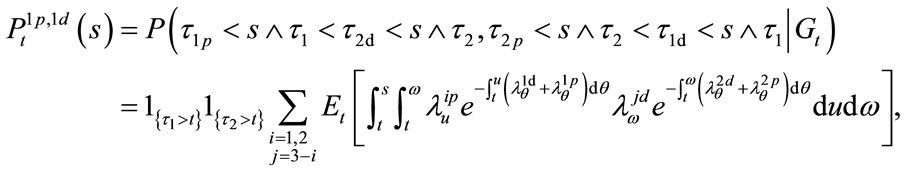
In order to price a basket LCDS, some probabilities need to be calculated as follows:
 : from time
 , the probability of one prepaying (defaulting) and the other surviving before time
![]() ;
;
 : from time
 , the probability of one prepaying (defaulting) in anterior to the other defaulting (prepaying) before time
![]() ;
;
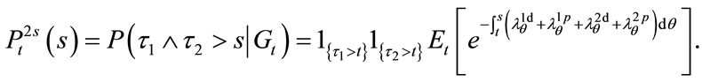
 : from time
 , the probability of prepaying (defaulting) of both loans before time
![]() ;
;
 : from time
 , the probability of surviving of both loans before time
![]() ;
;
According to the assumptions we can obtain the expressions for the probabilities above as follows (here we take ):
):
 (8)
(8)
 (9)
(9)
 (10)
(10)
 (11)
(11)
 (12)
(12)
 and
and 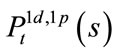 can be calculated similarly, but no use for the pricing formula.
A basket LCDS pricing formula can thus be obtained with the help of the basic pricing model of a single-name of LCDS in [13]. We assume that the expiration time of the contract is![]() , the spread at time
, the spread at time  is
is , the face or fair value of the reference loan is F. The days of payment are assumed to be
 , with
  representing the sum of periods. The interval between two paying dates is
 . The current price of an LCDS contract is the difference between the expected present values of protection and premium, in other words,
By applying the cash flow discounting method to the probability expressions Equations (8)-(12), the present values of insurance spreads and compensation can be obtained as follows:
 (13)
(13)
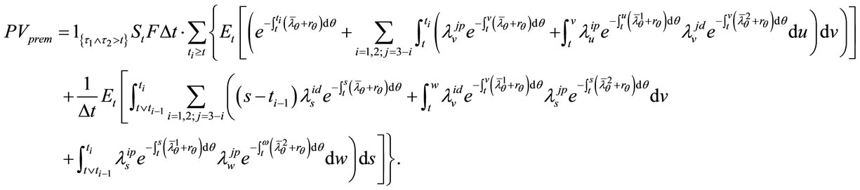 (14)
(14)
where  is the recovery rate when default occurs and is assumed to be a constant,
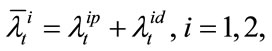
The fair price of this basket LCDS can be obtained by letting 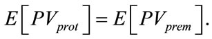
3.2. Model Solution
The key of pricing basket LCDS is to calculate the probabilities Equations (8)-(12), so that it is necessary to model default and prepayment intensities, which are negative correlated and both non-negative processes. We assume them to satisfy SDEs as follows:
 (15)
(15)
where  and
and  are all non-negative constants; The process of risk free spot interest rate,
  , is the systematic risk factor in this model, and
  are non-systematic risk factors.
  and
and  are mutually independent and drove by CIR processes
 :
:
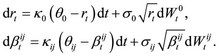 (16)
(16)
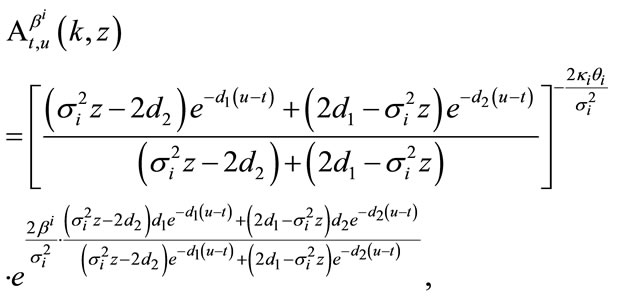
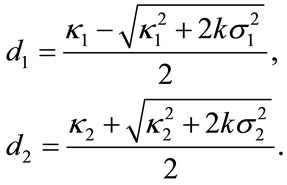
According to [9], the explicit formulas for probabilities Equations (8)-(12) can be written as functions of ,
,  and
and . The expression of
  is as the previous chapter, and the expression of
  and
and  are as follows:
 (17)
(17)
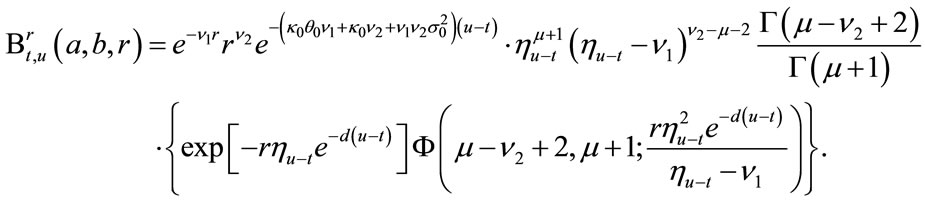 (18)
(18)
where  and
and  are the same as in the former chapter,
  is the gamma function, and
 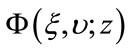 is a confluent hyper geometric function:
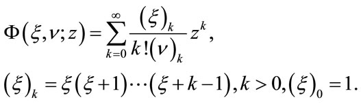 (19)
(19)
For the solving process of , for details please refer to [9,12-15]. In this way, the price of tworeference basket LCDS can be obtained explicitly.
3.3. Numerical Simulation
Based on the closed-form solution of two-reference basket LCDS obtained in the previous subsection, a calculation example is provided in this part, and the relevant parameter analysis is carried out. Thanks to the closedform solutions, the computation is relatively fast and efficient, but the calculation amount is much larger than that of single-name LCDS. In this simulation the basic parameters are set as follows if they are not specified:
The four pictures in Figure 3 are the theoretical prices of the basket LCDS, and the relationship between the price of basket LCDS and the initial value of the interest rate![]() , the reversion mean value
, the reversion mean value , the velocity of regression
  and the volatility
  are shown in the pictures respectively. It is distinctly shown in the charts that the price of this LCDS increases together with
![]() ,
,  or
or . Furthermore, the influence of the reversion mean value
  towards the price of the LCDS is relatively slight when the duration of the contract,
 ![]() , is small, and remarkable when
, is small, and remarkable when ![]() is big. This is similar with the phenomenon with single name LCDS. As for initial value of interest rate
is big. This is similar with the phenomenon with single name LCDS. As for initial value of interest rate![]() , this property isn’t evident, and the volatility
, this property isn’t evident, and the volatility  influences the price in a contrary way. As is the case of single name LCDS, the price is least sensitive to the reversion speed
 , and increases together with
 .
.
All the four pictures show an increase-decrease tendency of the basket LCDS price with the growth of terminal![]() , which are different from the ones of the single-name LCDS. The reason lies in the fact that the contract won't be terminated unless both loans are prepaid, which reduces the termination probability by prepayment. As the duration of the contract increases, the expected number of payment increases as well, while the number of loans under protection does not change. As a result,
, which are different from the ones of the single-name LCDS. The reason lies in the fact that the contract won't be terminated unless both loans are prepaid, which reduces the termination probability by prepayment. As the duration of the contract increases, the expected number of payment increases as well, while the number of loans under protection does not change. As a result,
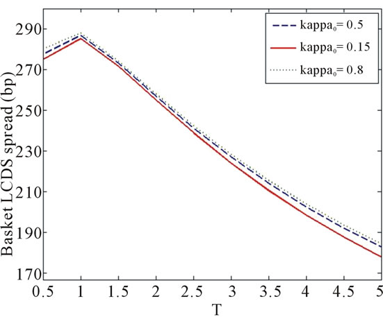
Figure 3. Sensitivity between the price of basket LCDS and .
.
the spread of the basket LCDS decreases.
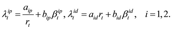
As the method employed with single name LCDS, only the ratio of the system risk factor in  and
and  is changed. As a result, the values of these intensities remain almost unchanged. It can be indicated from Figure 4 above that the price of basket LCDS will increase as the increment in correlation between prepayment and default.
4. Large-Scale Basket LCDS Pricing
In the case that the asset pool contains  prepayable loans,
  intensity processes should be taken into consideration. Here we still use
  and
and 
 to represent the prepayment and default intensity processes of loan i respectively, and define the probability space
  as the preceding text.
In the case with prepayable nth-to-default LCDS, the contract will be terminated and indemnity is made if the total number of default loans in the asset pool reaches![]() . If less than
. If less than ![]() loans default in the pool and the other loans are all prepaid, the contract will also be stopped with no compensation. Seen from time
loans default in the pool and the other loans are all prepaid, the contract will also be stopped with no compensation. Seen from time , the probability of
 ![]() loans are prepaid while m loans survive
loans are prepaid while m loans survive
 before time
 ![]() is assumed to
is assumed to 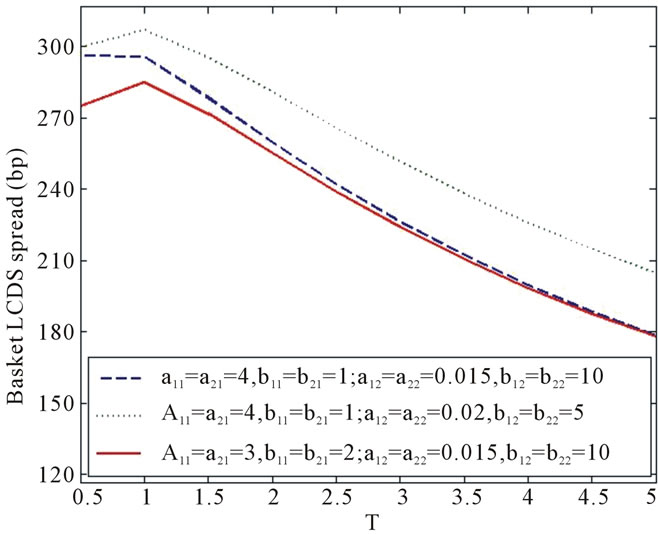
Figure 4. Basket LCDS premiums vs correlations between prepayment and default.
be . Especially, all the loans survive when
 , so
, so  is the joint survival probability of all
  loans. According to the assumptions in the framework of reduced form method, the expressions of these probabilities above are as follows: (here
 )
)
 (20)
(20)
 (21)
(21)
where  denote prepayment and default sequences respectively, and

The solution progress of  can be divided into
  time intervals. Suppose that
  are the moments of the last three credit events. By the technique used in pricing two-reference LCDS, from time
  o
o , the expectation
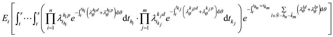
can be rewritten as
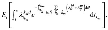
And from  to
to , the expectation can be written as

Same as the case with two-reference LCDS,  and
and 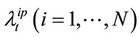 are modeled as follows:
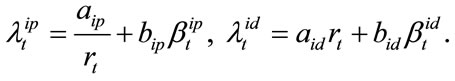 (22)
(22)
 are all non-negative constants. The two expectations can be expressed as functions of
  The other intervals can be dealt with in the same way. Thus the explicit expression of Equation (20) can be obtained, and the price prepayable nth-to-default LCDS can be derived.
Although the model in this chapter provides us an explicit solution, the large scale of calculation prevents us from evaluating it directly. Here only the outcomes by Monte Carlo stimulation are demonstrated. It is indicated in Figure 5 that the price of a first-to-default LCDS with an asset pool of two loans (with an expiration of over two years) is lower than that of a single-name LCDS, which concords the property shown in the model and result in Sections 3.2 and 3.3.
According to Figures 6 and 7, the price of firstto-default basket LCDS (corresponding to the case ) is decreasing with the enlargement of expiration
![]() . In the case when
. In the case when , the price of second-to-default basket LCDS is first increasing then decreasing along with
![]() . And the price of fourth-to-default basket LCDS is increasing along with terminal
. And the price of fourth-to-default basket LCDS is increasing along with terminal![]() . In summary, the price
. In summary, the price
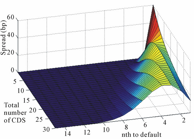
Figure 5. Price surface of large scale nth-to-default LCDS.
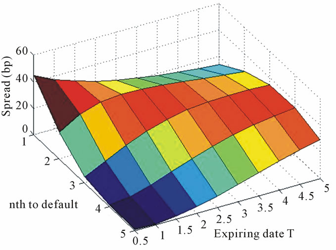
Figure 6. Price surface of nth-to-default LCDS (N = 30).
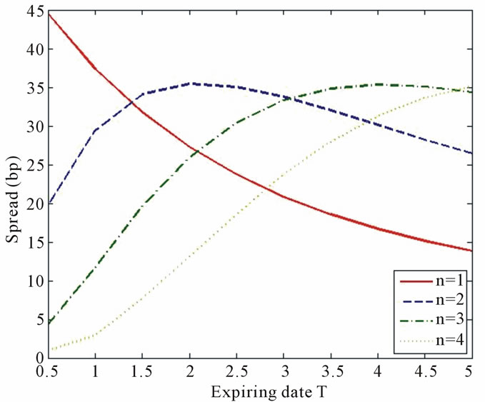
Figure 7. Relationship between nth-to-default basket LCDS and n (N = 30).
of basket LCDS first decreases then increases with terminal time ![]() as
as ![]() increases, and this coincides the conclusions in 3.3. The reason of this phenomenon may lie in this fact: we have assumed from the beginning that the LCDS will only be terminated due to prepayment when the living loans are all prepaid while the number of default loans is smaller than
increases, and this coincides the conclusions in 3.3. The reason of this phenomenon may lie in this fact: we have assumed from the beginning that the LCDS will only be terminated due to prepayment when the living loans are all prepaid while the number of default loans is smaller than![]() . As a result, the probability to close the contract by prepayment is rather small when
. As a result, the probability to close the contract by prepayment is rather small when ![]() is small, and the surviving probability of the contract is larger with larger
is small, and the surviving probability of the contract is larger with larger![]() . The augmentation in the times to pay spreads reduces the spread rate. Contrarily, the prepayment probability increases and the number of payment decreases, resulting in an increasing spread rate.
. The augmentation in the times to pay spreads reduces the spread rate. Contrarily, the prepayment probability increases and the number of payment decreases, resulting in an increasing spread rate.
5. Conclusion
In this paper, a single factor model with CIR process used in pricing a single-name LCDS is extended for pricing a basket CDS and LCDS. The model is under reduced form framework, where the prepayment and default are two negative correlated processes following factor CIR processes. Pricing formulas for basket CDS, two-reference basket LCDS and large-scale basket LCDS are established and calculated. The first two prices are presented numerical examples analytically while the last one is shown by Monte Carlo simulation. From the results, analysis on parameters is carried on.
REFERENCES
- H. H. S. Shek, S. Uematsu and W. Zhen, “Valuation of Loan CDS and LCDX,” Stanford University, Stanford, 2007. http://papers.ssrn.com/sol3/papers.cfm?abstract_id=1008201
- P. Dobranszky and W. Schoutens, “Generic Levy OneFactor Models for the Joint Modeling of Prepayment and Default: Modeling LCDX,” Katholieke Universiteit Leuven, Leuven, 2008. http://papers.ssrn.com/sol3/papers.cfm?abstract_id=1008201.
- P. Collin-Dufresne and J. P. Harding, “A Closed Form Formula for Valuing Mortgages,” The Journal of Real Estate Finance and Economics, Vol. 74, No 2, 1999, pp. 133-146. doi:10.1023/A:1007879422329
- J. B. Kau, D. C. Keenan and A. A. Smurov, “ReducedForm Mortgage Valuation,” University of Georgia, Georgia, 2004. http://www.terry.uga.edu/realestate/docs/reducedform082504.pdf
- J. M. Ma and J. Liang, “Valuation of Basket Credit Default Swaps by Partial Differential Equation Method,” Applied Mathematics a Journal of Chinese Universities, Vol. 23, No. 4, 2008, pp. 427-436.
- T. Wang and J. Liang, “The Limitation and Efficiency of Formula Solution for Basket Default Swap Based on Vasicek Model,” Systems Engineering, Vol. 27, No. 5, 2009, pp. 49-54.
- J. Liang, J. M. Ma, T. Wang and Q. Ji, “Valuation of Portfolio Credit Derivatives with Default Intensities Using the Vasicek Model,” Asia-Pacific Financial Markets, Vol. 18, No. 1, 2011, pp. 33-54. doi:10.1007/s10690-010-9119-z
- W. Zhen, “Valuation of Loan CDS under Intensity Based Model,” Stanford University, Stanford, 2007. http://www.defaultrisk.com/pp_crdrv144.htm
- J. Liang and T. Wang, “Valuation of Loan-Only Credit Default Swap with Negatively Correlated Default and Prepayment Intensities,” International Journal of Computer Mathematics, in Press.
- J. Liang and Y. J. Zhou, “Valuation of a Tranche Loan Credit Default Swap Index,” Technology and Investment, Vol. 2, No. 4, 2011, pp. 240-246. doi:10.4236/ti.2011.24025
- Y. J. Zhou and J. Liang, “Valuation of a Basket Loan Credit Default Swap,” International Journal of Financial Research, Vol. 1, No. 1, 2010, pp. 21-29.
- Y. Wu and J. Liang, “Valuation of Loan Credit Default Swaps Correlated Prepayment and Default Risks with Stochastic Recovery Rate,” International Journal of Financial Research, in Press.
- J. Liang, T. Wang and X. Yang, “Single Name LCDS Pricing and Related CVA Calculation regarding Counterparty Default,” Tongji University, Shanghai, 2011.
- X. S. Qian, L. S. Jiang, C. L. Xu and S. Wu, “Explicit Formulas for Pricing of Mortgage-Backed Securities in a Case of Prepayment Rate Negatively Correlated to Interest Rate,” Unpublished, 2009.
- T. R. Hurd and A. Kuznetsov, “Explicit Formulas for Laplace Transforms of Stochastic Integrals,” Mcmaster University, Hamilton, 2006. http://www.math.mcmaster.ca/tom/StochIntHurdKuzn.pdf