Wireless Engineering and Technology
Vol.3 No.4(2012), Article ID:24191,4 pages DOI:10.4236/wet.2012.34032
State Estimation over Customized Wireless Network
![]()
1Young Researchers Club, Zarghan Branch, Islamic Azad University, Zarghan, Iran; 2School of Electrical and Computer Engineering, Shiraz University, Shiraz, Iran.
Email: vahid.naghavi@yahoo.com
Received May 11th, 2012; revised June 10th, 2012; accepted June 20th, 2012
Keywords: Estimation; Customized Wireless Network; Kalman Filtering; Time Varying Delay
ABSTRACT
In this paper the state estimation techniques are investigated over customized wireless network for a continuous-time plant. It is assumed that the plant is connected to the controller over the proposed network. The feedback control over wireless networks includes limited bandwidth, time-varying and unknown delays with a high probability of data loss. Reasonably, some of these issues are deduced from the wireless networks structures. In order to deal with these problems the customized wireless network architecture is proposed for this Wireless Networked Control System (WNCS) and the problem of transmission delays and packet losses which induced by this scheme is studied. The time-varying delays of the TCP based shared network is estimated by fuzzy state estimation technique. Thereafter the kalman filtering is applied to address the problem of optimal filtering for this continuous-time plant with time-varying delays. The re-organized innovation analysis approach is applied to tackle the network induced time-varying delays. The simulation results show the applicability of the proposed approach.
1. Introduction
Networked control systems (NCSs) are systems in which control loops are closed over a real-time communication network. The fact that controllers, sensors, and actuators are not connected through point-to-point connections, but through a multipurpose network offers advantages, such as increased system flexibility, ease of installation and maintenance, and decreased wiring and cost. Further development and research in NCSs were boosted by the tremendous increase in the deployments of wireless systems in the last few years. Despite the many advantages, a distributed control system over a network may offer, the insertion of a communication network in the feedback loop will in general introduce more complexities in the system. For example, as a direct consequence of the finite bandwidth for data transmission over networks, time-delay is inevitable in networked systems where a common medium is used for data transfers. In addition to transmission delays, some packets can also be lost during transmission. See [1-2] for overview of recent research on NCSs.
This paper deals with continuous-time plants. The plant is remotely controlled over the customized wireless networked. In other hand feedback control over wireless networks include limited bandwidth, time-varying and unknown delays and a high probability of data loss. This makes WNCS much more challenging for control design than the conventional wired alternative; reasonably, some of these issues deduce from the wireless networks structures which we should address them in our design procedure. In order to make a practical sense, the customized wireless network architecture is proposed for this Wireless Networked Control System (WNCS) and the problem of transmission delays and packet losses which induced by this scheme is studied. Meanwhile the timevarying delay of the TCP based shared network is estimated by fuzzy state estimation technique ([3-4]). Thereafter the kalman filtering is applied to address the problem of optimal filtering for this continuous-time system where the observations are communicated to the estimator via an unreliable channel resulting in timevarying delays. The filtering problem for NCSs has received much attention during the past few years ([5-7]). In [8] the re-organized innovation analysis approach is proposed for linear estimation [8], which is based on projection and a re-organized innovation sequence. This technique is adopted in [9] to address the problem of Kalman filtering for continuous-time systems with timevarying delay. We apply the proposed approach in [9] to tackle the network induced time-varying delay for optimal estimation of the states in NCS framework. The simulation results show the applicability of the proposed approach.
The organization of the paper is as follows. In Section 2, the customized wireless networks architecture is proposed. Section 3 describes the optimal estimation problem for continuous time linear systems with time-varying measurement delay. Thereafter in Section 4 the design procedure of minimum-variance filtering problem with multiple-step measurement delays was investigated via the Kalman filtering problem with delayed measurement. The simulation results in Section 5 illustrate the applicability of the proposed filtering schemes. Finally we give our conclusions in Section 6.
2. Proposed Customized Wireless Networks Architecture
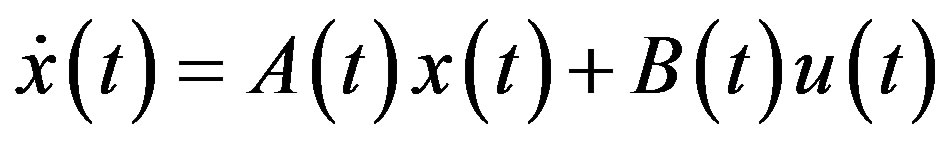
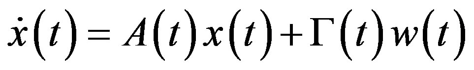
Consider the wireless networked control system setup in Figure 1; the plant is a linear time-variant continuoustime system as follows:
 (1)
(1)
where  are the states and input vectors.
  and
and  are time-varying matrices with proper dimensions.
The plant is remotely controlled over the customized wireless networked. As it is shown in Figure 2 we have three types of networks in the proposed architecture which can be described as follow:
1) Wireless Local Area Network (WLAN) contains of sensors and access point (WLAN1).
2) The TCP based shared Network i.e. Internet.
3) WLAN contains of actuators and access point (AP). (WLAN2).
Remark 1: One can use two different access points for WLAN1 and WLAN2 to prevent interference between these channels. In addition it can support sensors and actuators which located in separated areas.
Remark 2: The standard IEEE 802.11 has two basic modes of operation; 1) Ad hoc mode enables peer-to-peer transmission between mobile units; 2) Infrastructure mode in which mobile units communicate through an access point that serves as a bridge to a wired network infrastructure is the more common wireless LAN application. WLAN1 and WLAN2 are following standard IEEE 802.11 as infrastructure mode.
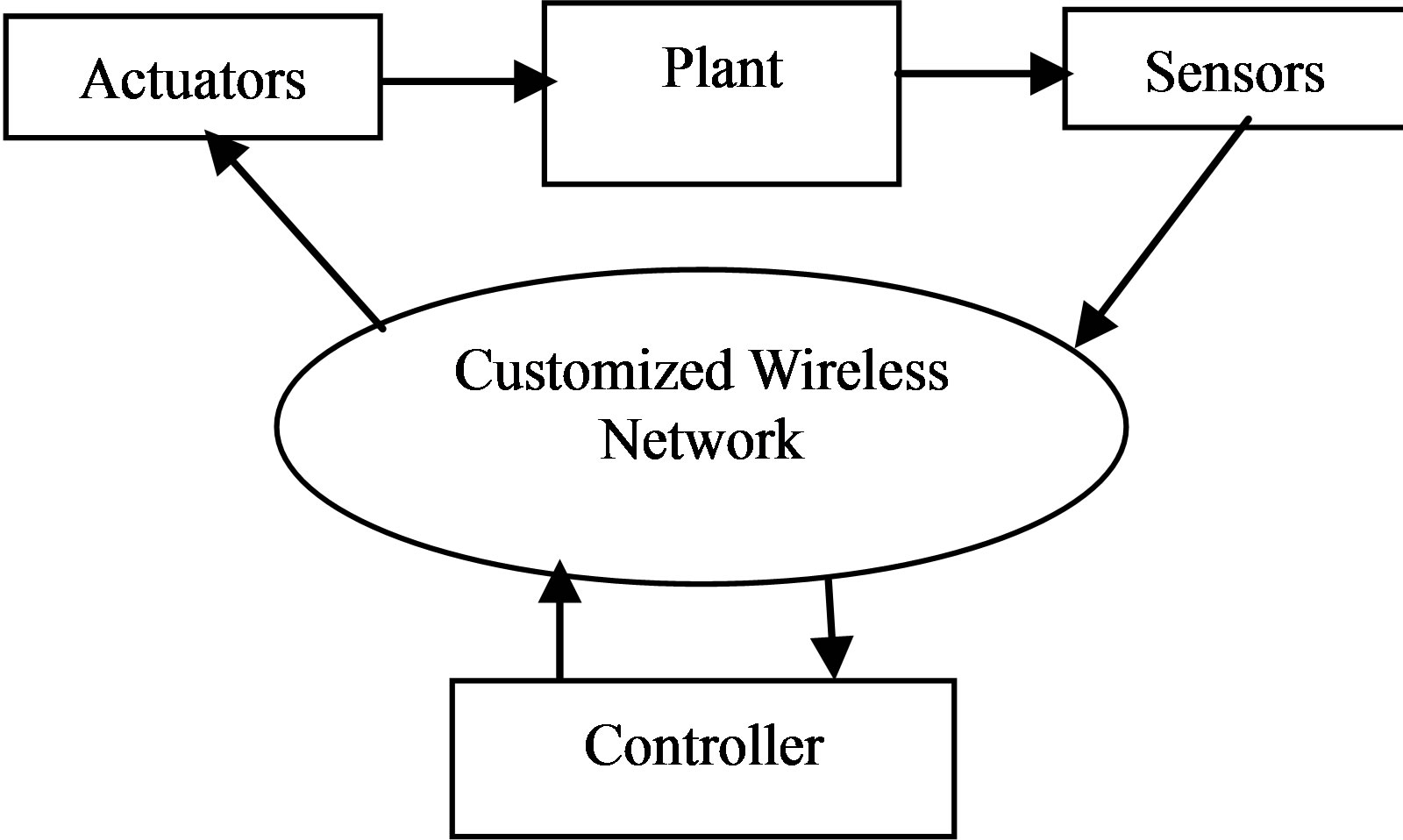
Figure 1. The wireless networked control system setup.
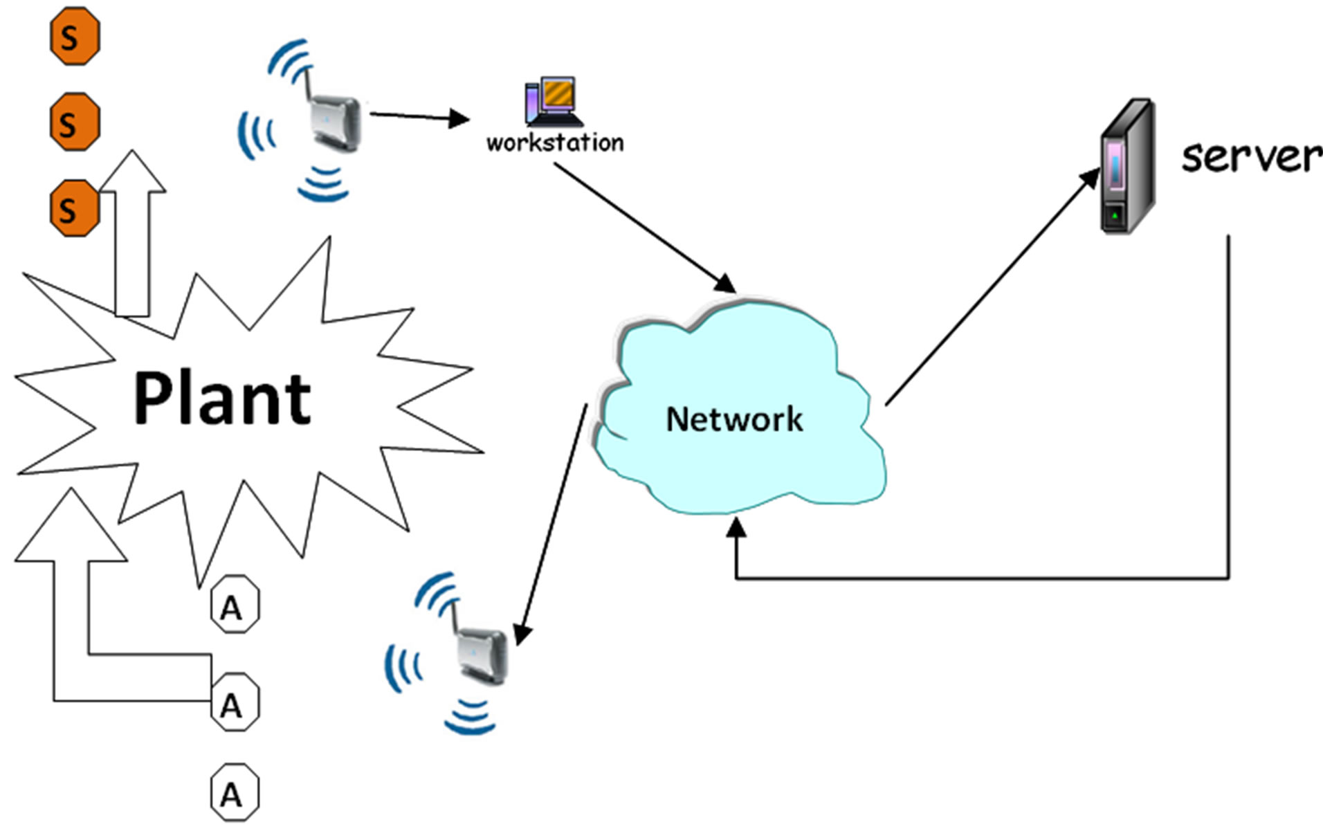
Figure 2. Proposed customized wireless networks architecture.
2.1. Characteristics of WLAN1
There are three basic principles in multiple access, FDMA (Frequency Division Multiple Access), TDMA (Time Division Multiple Access), and CDMA (Code Division Multiple Access). All three principles allow multiple users to share the same physical channel. But their technologies differ in the way user sharing the common resource. In our case the sensors are timedriven and the sampling time is constant. So we propose to use TDMA method, such method allows the users to share the same frequency channel by dividing the signal into different time slots. Each user takes turn in a round robin fashion for transmitting and receiving over the channel. In TDMA users can only transmit in their respective time slot. Unlike TDMA, in CDMA several users can transmit over the channel at the same time.
In other word, TDMA technology separates users according to time; it ensures that there will be no interference from simultaneous transmissions, therefore it guaranties that no packet loss and congestion will occur. This result is valid while sensors are located in the range of transmission area. In addition it provides users with an extended battery life, since it transmits only portion of the time during conversations. This could be also applicable for us because our proposed scheme is based on wireless networks.
Although there are no packet losses, TDMA method has a bit of delay for transmitting packets of data across the channel. This delay deduces from the waiting time which is used in TDMA algorithm and can be calculated as a constant delay in our model ( ).
).
In other hand, we need time synchronization in TDMA method. Timing Synchronization Function (TSF) is specified in IEEE 802.11 wireless local area network (WLAN) standard to fulfill this purpose. On a commercial level, industry vendor assumes the 802.11 TSF’s synchronization to be within 25 microseconds. We add this time as a time synchronization delay in the proposed scheme ( ).
).
2.2. Characteristics of WLAN2
The most significant feature of WLAN2 is that the actuator nodes only receive data and just send an acknowledge packet (ACK) to access point. So against WLAN1 we don’t need to define a special policy for media access control (like TDMA) to prevent congestion between senders, and access point can manage and control data transmission according to standard IEEE 802.11.
While the access point tries to send data to actuators, it should wait equal to DIFS time interval. In the DCF protocol in IEEE 802.11 all stations should check the status of wireless medium before getting into transmission level. If the medium is continuously idle for DCF Inter frame Space (DIFS) duration then it is allowed to transmit a frame.
After data was sent, receiver should send an ACK to AP. This ACT should wait just for SIFS time interval. Short Inter-frame Space (SIFS), is the small time interval between the data frame and its acknowledgment. SIFS is found in IEEE 802.11 networks. They are used for the highest priority transmissions enabling stations with this type of information to access the radio link first. Figure 3 shows a sender accessing medium and sending its data.
According to the fact that in our scheme the actuators don’t send data packets to the receiver, we can ignore the back-off time in this network with standard IEEE 802.11 and customize our WLAN without this time interval. The total induced time delay in WLAN2 is the sum of SIFS, DIFS and ack time (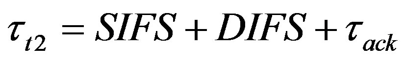 ).
).
2.3. TCP Based Shared Network
In TCP based shared networks, most of resources are shared between many other users i.e. internet users, and the routes of packets are unpredictable over routers on these networks. Consequently it is impossible to determine exactly the dynamics of such networks. One problem that must be resolved when using a Transmission Control Protocol (TCP) is how to deal with timeouts and retransmissions.
In telecommunications, the RTT is the length of time it takes for a signal to be sent plus the length of time it takes for an acknowledgment of that signal to be received. The RTT was originally estimated in TCP by:
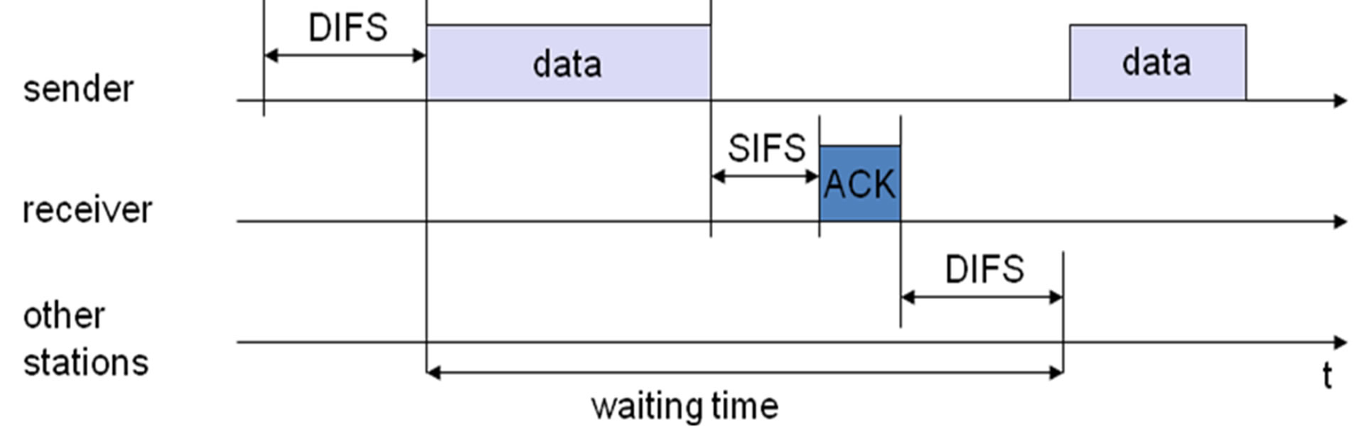
Figure 3. A sender accessing medium and sending its data.
 (2)
(2)
where, SRTT is the estimated RTT and α is the network related weighting parameter. We can use RTT as a measure of time delay in TCP network, but according to the dynamic of the network, the induced time delay is timevarying and depends on the interaction of multiple users on the network ( ). To illustrate the time-varying behavior of RTT, the real-time records of the RTT over Internet are shown in Figure 4.
In Equation (2) α parameter is generally unknown in practice, so the fuzzy state estimation is proposed to estimate the RTT in Section 2.4.
2.4. Fuzzy State Estimation
The mathematical formulation for a fuzzy state estimator is depicted in Equation (2). The estimator is controlled by the parameter α which is the weight given to the past history. The value of α can be determined by a knowledge of the network and error variances. In a network with a high signal-to-noise ratio, α should be large so that the past estimated RTT is given more weight and the transient changes in measurements are ignored.
On the other hand, in a network with a low signalto-noise ratio, the past estimated could vary, and the measurements would then reflect changes in both past estimation and the observation noise. By choosing lower value of α in such a case, the estimator quickly tracks changes in past estimation. Therefore, α adapts to the change, allowing us to obtain an optimal estimation of states at all times. Fuzzy estimator requires: 1) specification of the rules in terms of linguistic variables; and 2) the membership functions which can be determined experimentally due to network structure. For example the rules in the estimator are given as follow:
Rule 1. If error is low, then α is high.
Rule 2. If error is medium, then α is medium.
Rule 3. If error is high, then α is low.
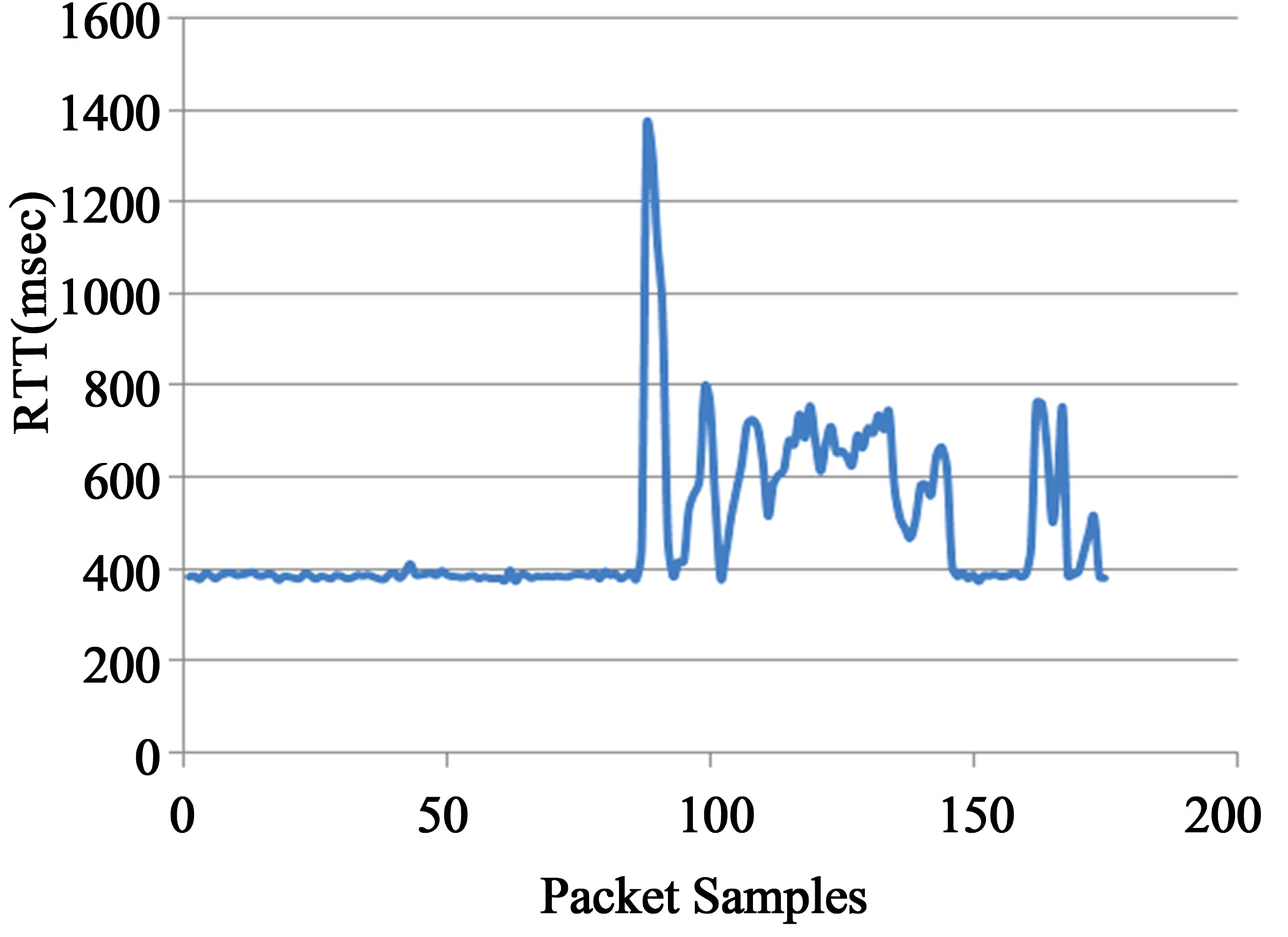
Figure 4. The real-time records of the RTT over internet.
and the membership functions of the error and α are illustrated in Figure 5.
Remark 3: In the case that the sensors are all collected at a single node, it is unlikely that their information would need to be split into multiple packets. Most control networks have a minimum packet size so that small packets don’t get ‘‘lost’’ on the network. For example, a DeviceNet packet can have between 0 and 8 bytes of data and an Ethernet packet can have between 46 and 1500 bytes of data, in addition to the headers, addressing information, and other overhead that must be included to ensure correct delivery of the packet. Since most D/A and A/D cards use either 12 or 16 bits (2 bytes) to encode sensor/actuator data, several channels of data can easily be transmitted in a single packet. By using this method we can reduce the over-head of each packet and eventually decrease the total network traffic rate.
Remark 4: It is worth mentioning that the largest portion of the delay in practice is usually due to the device delay: the delay in sampling the variable of interest from the environment, encoding that data into a packet, and then transmitting that data across the network and need to be measured experimentally for network devices ( ).
).
Remark 5: Packet loss can be caused by a number of factors, including signal degradation over the network medium due to multi-path fading, packet drop because of channel congestion, corrupted packets rejected in-transit,
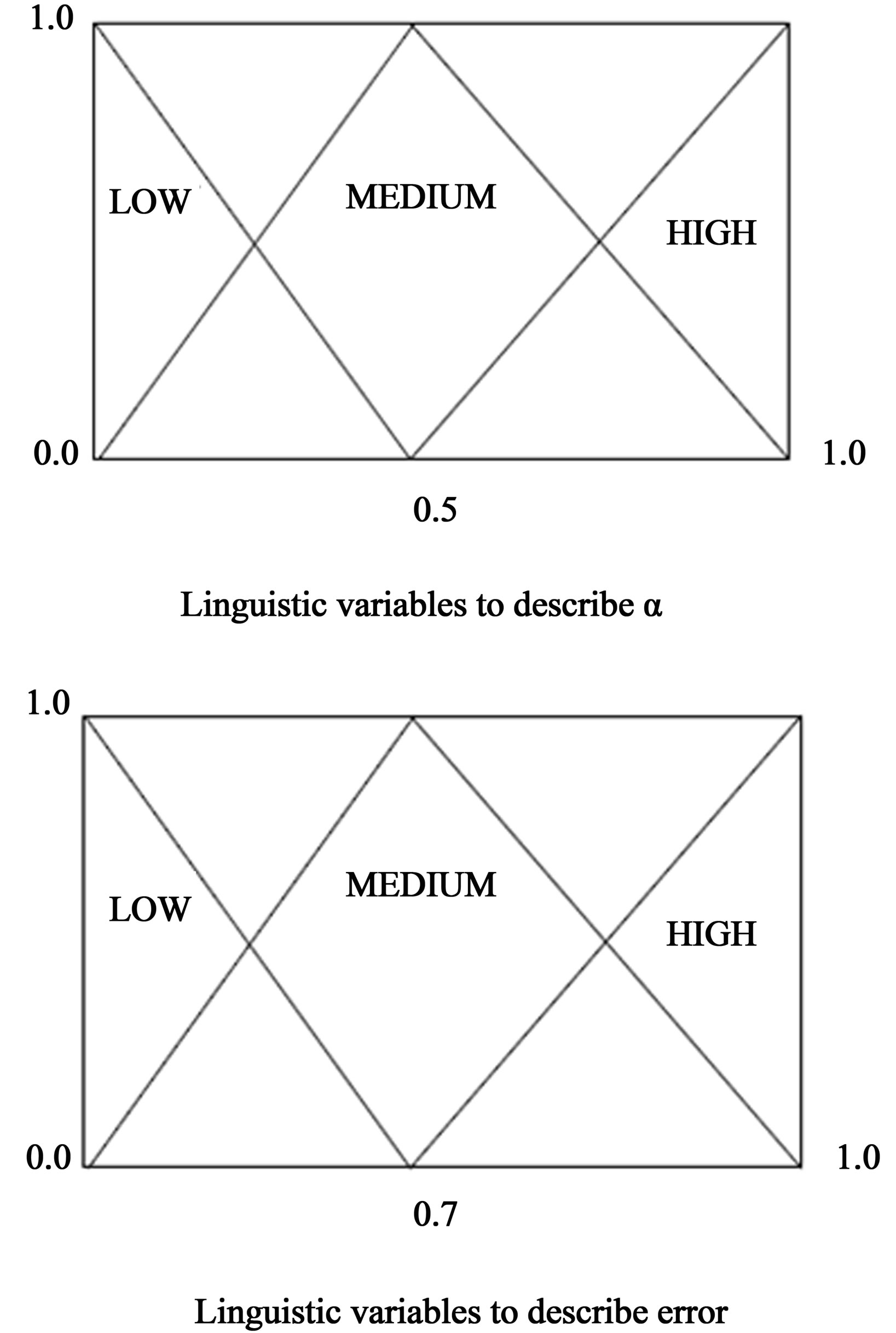
Figure 5. Membership function for error and α.
faulty networking hardware, faulty network drivers or normal routing routines. In our customized network WLAN1 and 2, according to our solution and customizetion, the reasons may cause packet losses include Signalto-noise ratio and distance between the transmitter and receiver but data packet dropout in TCP based shared network is unavoidable. In addition, it might be more advantageous to drop the old packet and transmit a new one than repeated retransmission attempt when packet collision occurs.
In the next section the kalman filtering is applied to address the problem of optimal filtering for the continuous-time system. The observations are communicated to the estimator via an unreliable channel resulting in timevarying delays. As it was mentioned in this section, we can assume that the time-varying delay is discrete and takes values from a finite set in other words, while the length of the delay that a packet has actually suffered upon arrival is assumed to be known exactly, we also assume that the delays may be different at different time instants.
3. Problem Formulation
Consider the continuous-time linear time-invariant model:
 (3)
(3)
 (4)
(4)
where  is the state vector,
  is the measured output, and
  and
and  are uncorrelated, zero-mean white noise processes with covariance matrices:
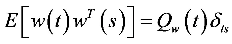 (5)
(5)
 (6)
(6)
and the initial condition satisfying the mean and covariance conditions:
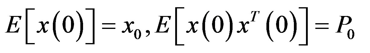 (7)
(7)
We assume that the plant is observable from the measured output .
.
Multiple-Step Measurement Delay Model and Formulation
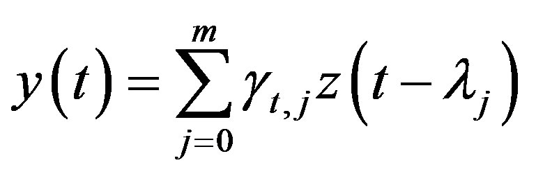
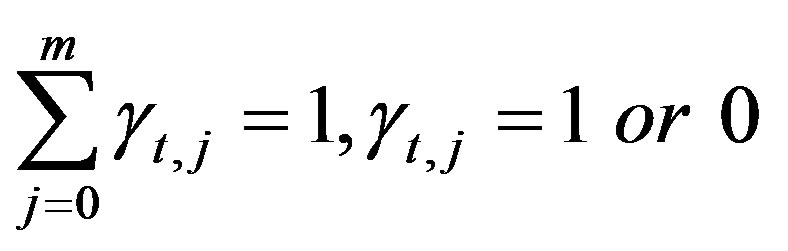
As in [9], we shall assume instead of , the observation may be delayed by a maximum of m samples. The system may then be represented as follows:
 (8)
(8)
 (9)
(9)
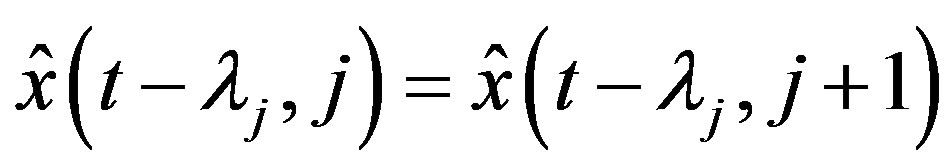
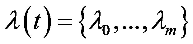 is the discrete time-varying delay and is known to the estimator.
  is the output observed at time
 . Note that
  corresponds to no sensor delay.
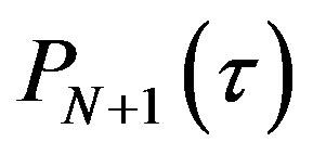
4. State Estimation with Multiple-Step Measurement Delays
4.1. Reorganised Observation and Innovations
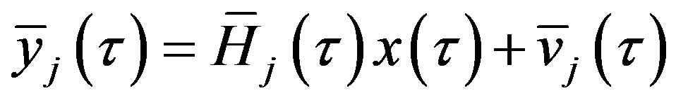
The observation Equation (8) can be rewritten equivalently as
 (10)
(10)
where
 (11)
(11)
with ,
, . It is readily known that
  are uncorrelated white noises with zero means and covariance
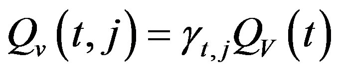 .
.
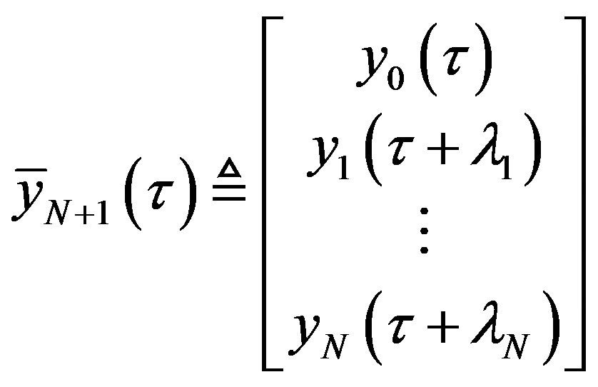
Let  denote all the observations possibly received at the estimator site at time t, then we have
 (12)
(12)
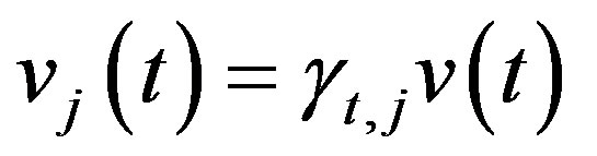
Note that the observation  is associated with states at different time instants which corresponding to different delays, the standard Kalman filtering is invalid for such estimation problems. To overcome the difficulties, we shall apply the reorganized innovation analysis approach. We first reorganized the observation as follows:
For 
 (13)
(13)
And for
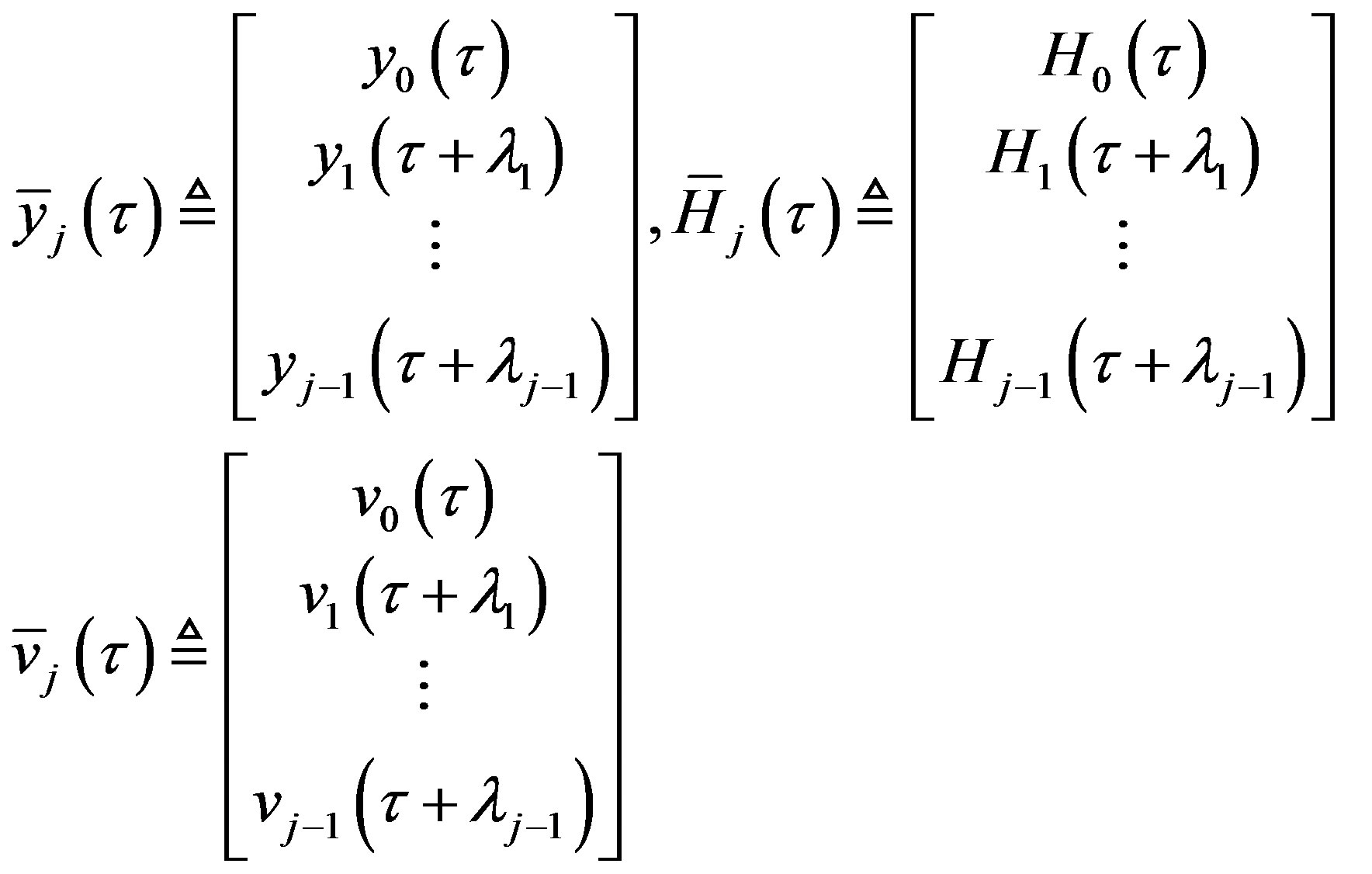 (14)
(14)
 satisfy the equation:
 (15)
(15)
It is readily known that  is a white noise with zero mean and covariance matrix
 (16)
(16)
Remark 6: Note that  in (14) is composed of different observations associated with the same state
 , so there is no delay existed any more.
4.2. Riccati Equations
As in the standard Kalman filter, we define the prediction error covariance matrices of the state as follows:
 (17)
(17)
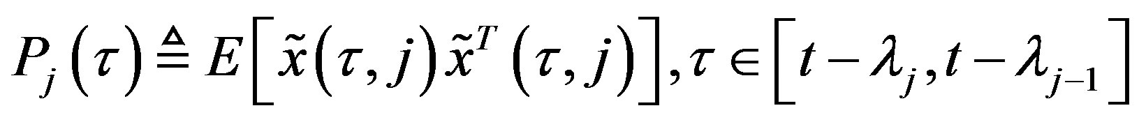 (18)
(18)
In Equations (16) and (17),  and
and  denote the state prediction errors covariance matrices of
  and
and  respectively, and they can be computed according to the following equations 1) With the given initial value
 ,
,  can be obtained by solving the following Riccati equation.For
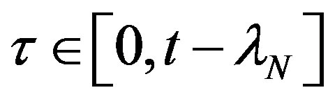 ,
,  is computed by
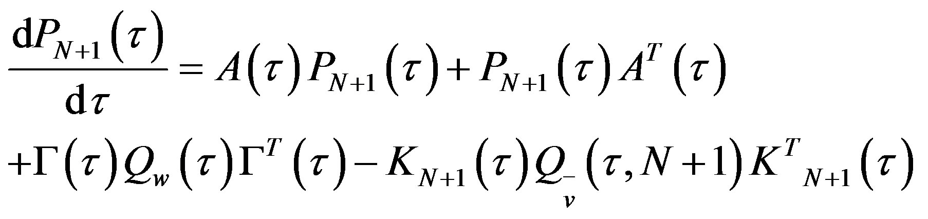 (19)
(19)
with 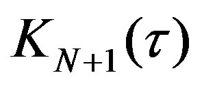 one solution of the following equation
 (20)
(20)
2) For ;
; 
 is computed by
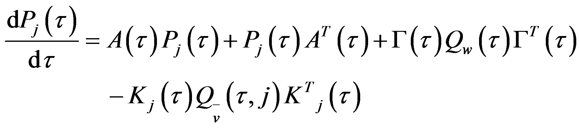 (21)
(21)
4.3. Optimal Filter
By applying the Riccati equations the optimal estimator 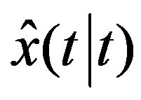 can be calculated as follows:
Step 1. Compute 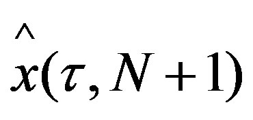 by using the differential equation
 (22)
(22)
with the given initial value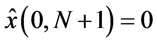 .
.
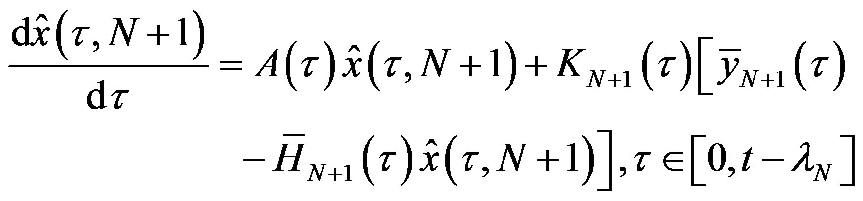
Step 2. Compute  for
for  by using the differencial equation
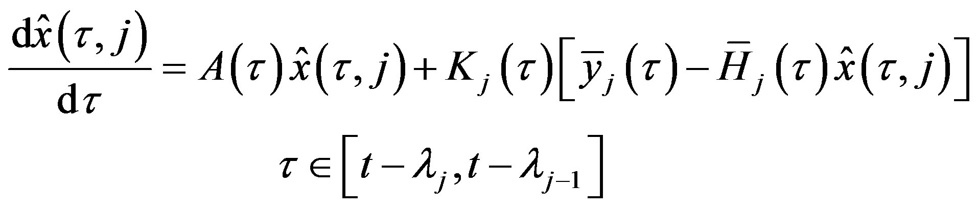 (23)
(23)
with the obtained initial value
 .
.
Step 3. Compute  from step 2 for
 .
.
Remark 7: The computation procedure for  is summarized in a flow chart that shown in Figure 6.
5. Simulation Results
In this section, we present a simple example to illustrate the previous theoretical results. Consider a dynamic system with the following specifications
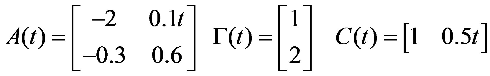
 and
and  are white Gaussian random variables with zero means and variance
  and
and  respectively.
 ,
, 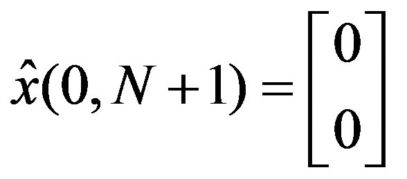 and
and 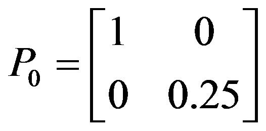
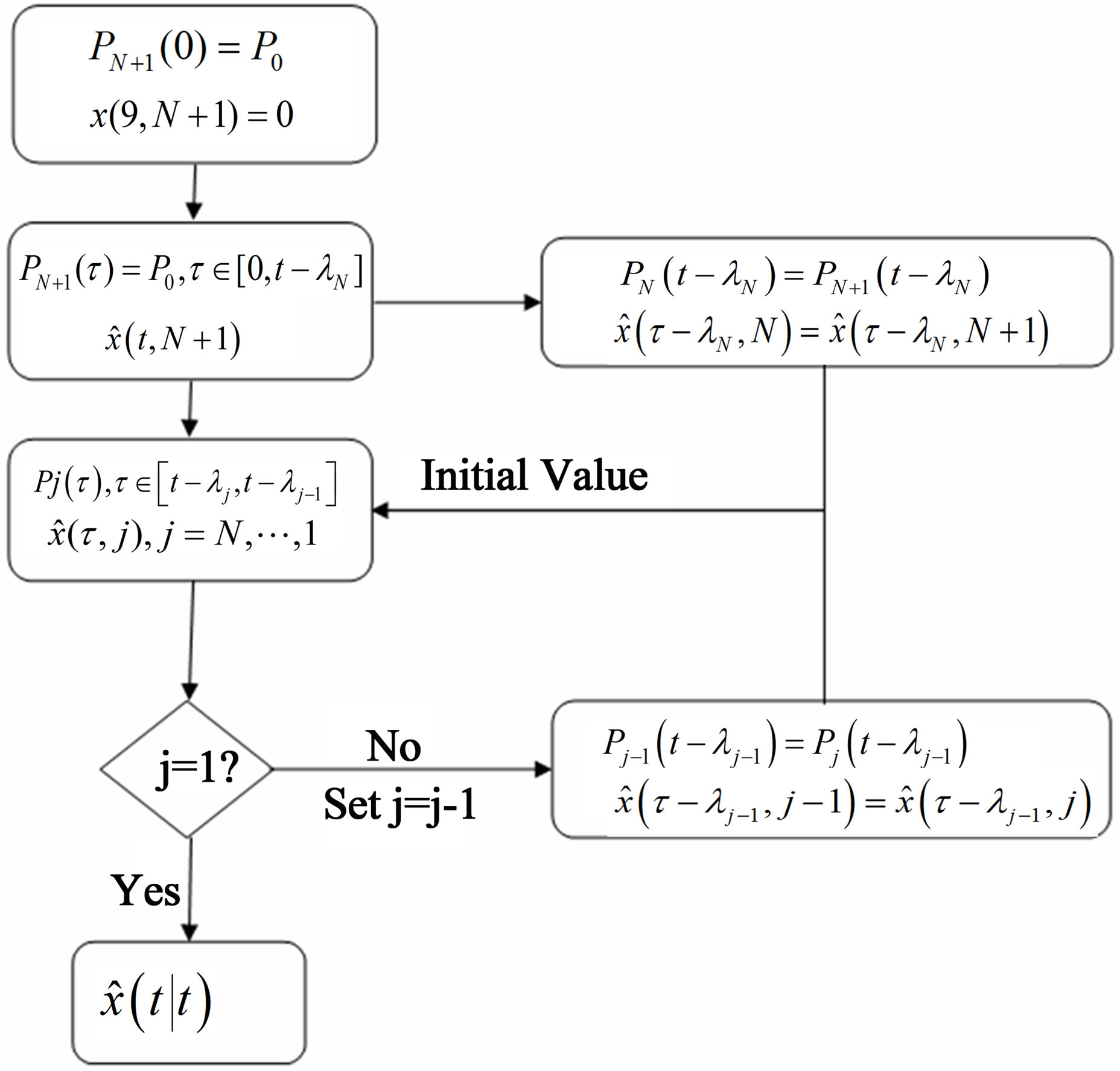
Figure 6. Flow chart for calculating .
.
are the initial values of ,
,  and
and , respectively. The time horizon is set to 5 and the sampling time
  to 0.01.
In the simulation, we consider a case of time varying delay as described in Figure 7. By applying the scheme proposed in Section 4, the optimal filter  can be obtained, as shown in Figures 8 and 9, where solid curves denote the true values and dotted curves denote the estimates.
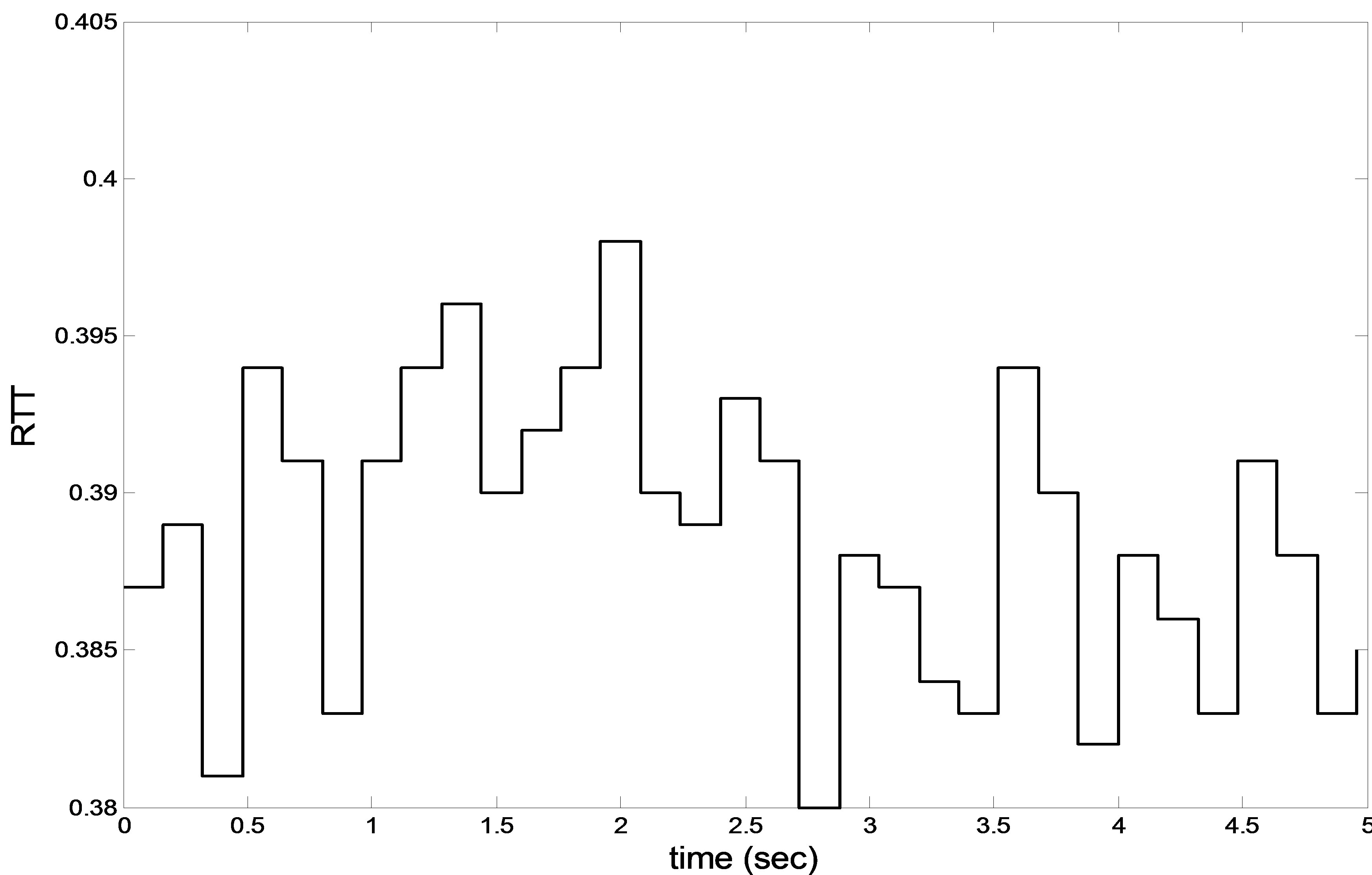
Figure 7. Time histories of RTT.
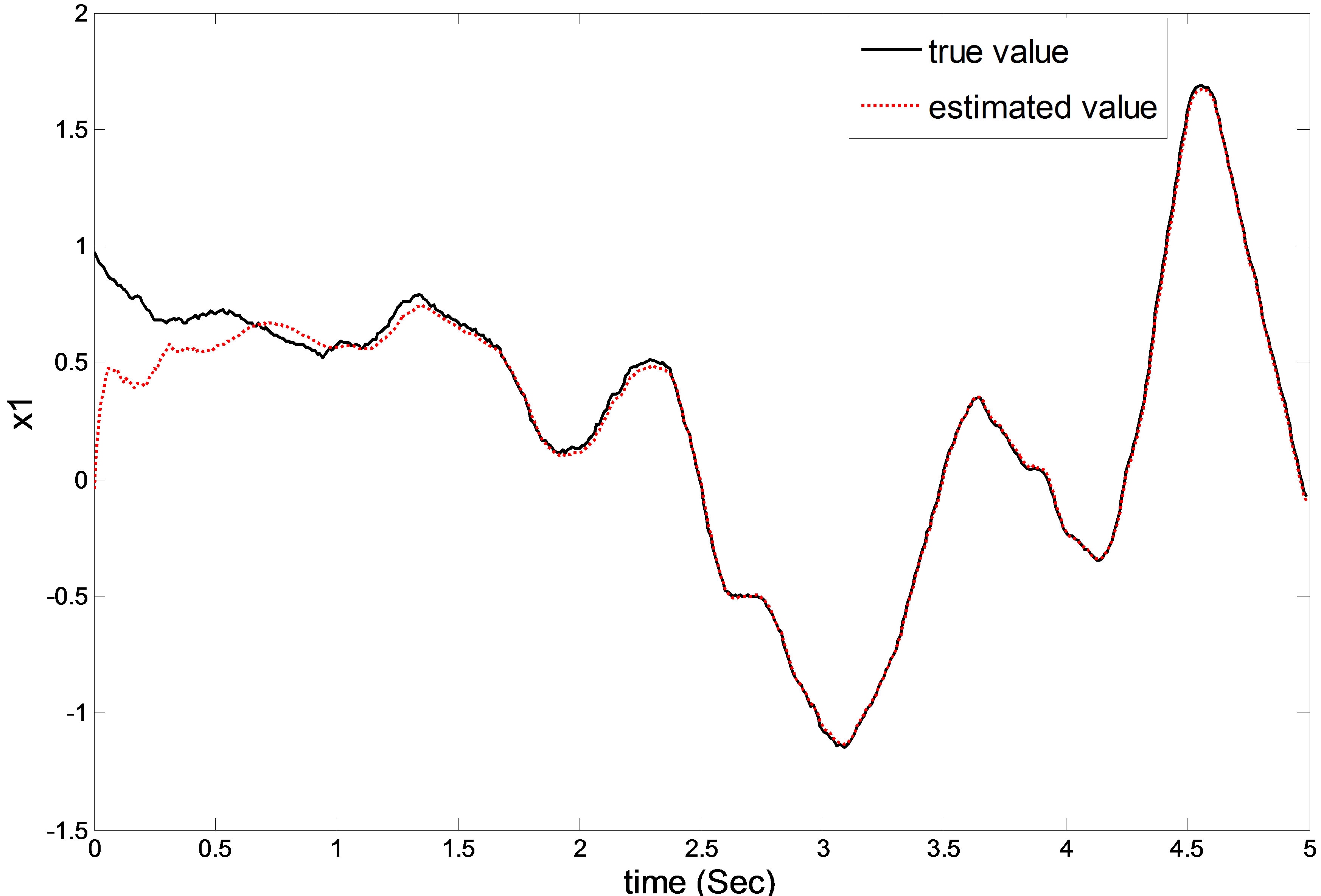
Figure 8. First state component  and filter
  under time varying delay.
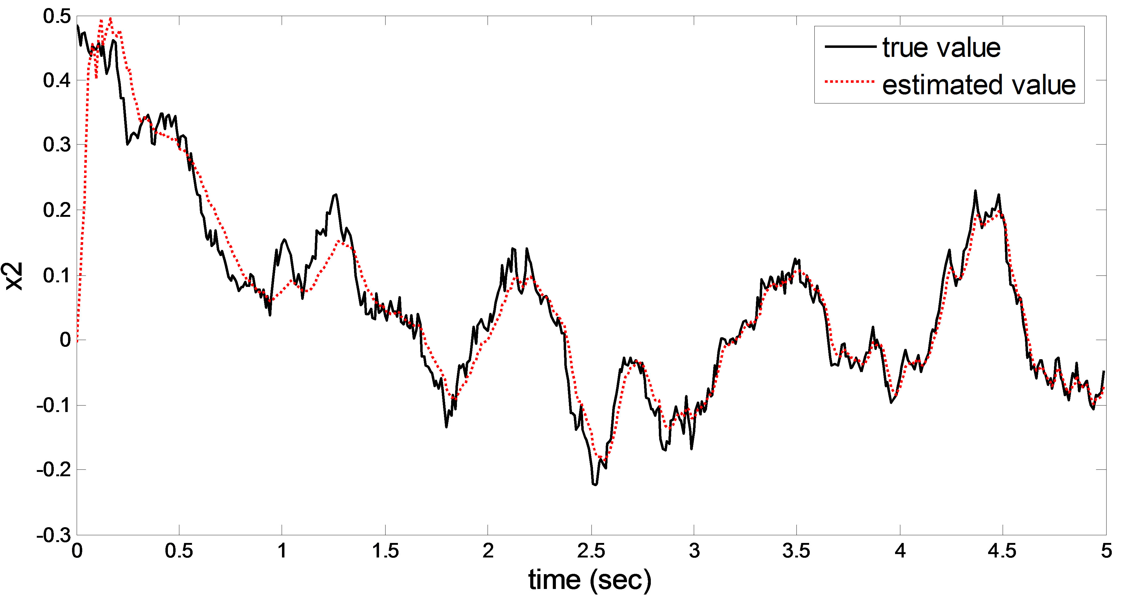
Figure 9. Second state component  and filter
  under time varying delay.
6. Conclusion
In this paper the state estimation techniques were investigated over customized wireless network for continuous-time plant in NCS framework. In order to deal with the network induced problems, the customized wireless network architecture was proposed and the problem of transmission delays and packet losses was studied. Thereafter the kalman filtering based on re-organized innovation analysis approach was applied for optimal state estimation in this framework. The simulation results illustrated the applicability of the proposed approach.
REFERENCES
- J. P. Hespanha, P. Naghshtabrizi and Y. Xu, “A Survey of Recent Results in Networked Control Systems,” IEEE Transactions on Automatic Control, Vol. 95, No. 1, 2007, pp. 138-162.
- R. A. Gupta and M.-Y. Chow, “Networked Control System: Overview and Research Trends,” IEEE Transactions on Industrial Electronics, Vol. 57, No. 7, 2010, pp. 2527- 2535.
- F. Shabaninia, “A Fuzzy-Logic-Supported Weighted Least Squares State Estimation,” Electric Power Systems Research Journal, Vol. 39. No. 1, 1996, pp. 55-60.
- F. Shabaninia, “State Estimation with Aid of Fuzzy Logic,” Proceeding of FUZZ-IEEE’96 Conference, Baton Rouge, 8-11 September 1996, pp. 947-952.
- M. Sahebsara, T. Chen and S. L. Shah, “Optimal H2 Filtering with Random Sensor Delay, Multiple Packet Dropout and Uncertain Observations,” International Journal of Control, Vol. 80, No. 2, 2007, pp. 292-301.
- S. Sun, L. Xie, W. Xiao and Y. C. Soh, “Optimal Linear Estimation for Systems with Multiple Packet Dropouts,” Automatica, Vol. 44, No. 5, 2008, pp. 1333-1342. doi:10.1016/j.automatica.2007.09.023
- M. Moayedi, Y. C. Soh and Y. K. Foo, “Optimal Kalman Filtering with Random Sensor Delays, Packet Dropouts and Missing Measurements,” Proceedings of American Control Conference, St. Louis, 10-12 June 2009, pp. 3405-3410.
- H. S. Zhang, L. H. Xie, D. Zhang and Y. C. Soh, “A Re-Organized Innovation Approach to Linear Estimation,” IEEE Transactions on Automatic Control, Vol. 49, No. 10, 2004, pp. 1810-1814. doi:10.1109/TAC.2004.835599
- W. Wang, H. Zhang and L. Xie, “Kalman Filtering for Continuous-Time Systems with Time-Varying Delay,” IET Control, Vol. 28, No. 4, 2009, pp. 590-600.