Journal of Environmental Protection
Vol.08 No.10(2017), Article ID:79248,25 pages
10.4236/jep.2017.810071
SO2 Oxidation Efficiency Patterns during an Episode of Plume Transport over Northeast India: Implications to an OH Minimum
Timmy Francis1,2*, Shyam Sundar Kundu3, Ramabadran Rengarajan1, Arup Borgohain3
1Physical Research Laboratory, Ahmedabad, India
2National Centre for Medium Range Weather Forecasting, Noida, India
3North Eastern Space Application Centre, Umiam, India
![]()
Copyright © 2017 by authors and Scientific Research Publishing Inc.
This work is licensed under the Creative Commons Attribution International License (CC BY 4.0).
http://creativecommons.org/licenses/by/4.0/


Received: August 2, 2017; Accepted: September 19, 2017; Published: September 22, 2017
ABSTRACT
Systematic monitoring of the fluctuations in atmospheric SO2 oxidation efficiency―measured as a molar ratio of to total SOx ( ), referred as S-ratio―have been performed during a major long range plume transport to northeast India (Shillong: 25.67˚N, 91.91˚E, 1064 m ASL) in March 2009. Anomalously low S-ratios (median, 0.03) were observed during the episode―associated with a cyclonic circulation―and the and SO2 exhibited unusual features in the ‘relative phase’ of their peaks. During initial days, when SO2 levels were dictated by the long range influx, the and SO2 variabilities were in anti-phase―for the differing mobility/loss mechanisms. When SO2 levels were governed by the boundary layer diurnality in the latter days, the anti-phase is explained by a ‘depleted OH level’―major portion being consumed in the initial period by the elevated SO2 and other pollutants. Simulations with a global 3D chemical transport model, GEOS-Chem (v8-03-01), also indicated ‘suppressed oxidation conditions’―with characteristic low S-ratios and poor phase agreements. The modelled OH decreased steadily from the initial days, and OH normalized to SO2―referred as OHspecific―was consistently low during the ‘suppressed S-ratio period’. Further, the geographical distribution of modelled OH showed a pronounced minimum over the region surrounding (20˚N, 95˚E) spanning parts of northeast India and the adjacent regions to the southeast of it―prevalent throughout the year, though the magnitude and the area of influence have a seasonality to it―with significant implications for reducing the oxidizing power of the regional atmosphere. A second set of measurements during January 2010―when prominent long range transports were absent―exhibited no anomalies, and the S-ratios were well within the acceptable limits (median, 0.32). This work highlights the GEOS-Chem model skill in simulating/detecting the ‘transient fluctuations’ in the oxidation efficiency, down to a regional scale.
Keywords:
Sulphur Dioxide, Sulphate, Atmospheric Oxidation, GEOS-Chem, OH Radical, Plume Transport

1. Introduction
Hydroxyl (OH) radicals many a time are aptly called ‘detergent of the atmosphere’, for the photochemical reactions initiated by them play crucial roles in the oxidation of huge quantities of natural and anthropogenic gases. The primary source of OH in any unpolluted lower tropospheric region is the photolysis of ozone, and a subsequent reaction with water vapour [1] . Secondary OH sources also exist in the troposphere, and the recycling of HO2 mainly by reaction with NO and O3, [2] is the prominent one.
Fluctuations in photolysis rate, relative humidity (RH) and ozone abundance can strongly affect the OH production, sometimes causing ‘transient changes in the oxidation capacity’ of atmosphere on a regional scale. The very short life times of OH for a high reactivity with carbon monoxide (CO) and hydrocarbons, especially methane (CH4) [3] [4] [5] , makes its concentration levels heavily dependent on the source and sink.
This paper reports an instance of ‘suppressed oxidation condition’ in the local atmosphere during a major plume transport episode detected [6] at our sampling site, Shillong, in north-east India―resulting in an anomalously low SO2 to conversion rate. While the molar ratio of to total SOx ( ), termed S-ratio, can be a good measure of the formation efficiency of in the atmosphere [7] , its variability is directly linked to the OH radical concentrations [8] [9] along with other factors such as boundary layer height, long range transport, dry deposition rate etc. The observations have been further compared with simulations employing a global 3D model of tropospheric chemistry, GEOS-Chem (v8-03-01).
2. Materials and Methods
2.1. Site Description
The sampling site, Shillong (25.67˚N, 91.91˚E, 1064 m ASL), located in the North-Eastern part of India, is characterized by a high annual rainfall (~2200 mm). While the high precipitation help retain a clean atmosphere via wet scavenging, occasional long range transport of pollutants many a time shows up clearly over the background in the atmospheric trace gas and aerosol measurements [6] [10] , making it an ideal site for studying long range pollution transport episodes. Its latitudinal location and high elevation provide it with a subtropical climate with mild summers and chilly to cold winters. The monsoon arrives by June and rains almost until the end of August, with low intensity precipitations sometimes showing up on either side of these months. The window of opportunity for most of the aerosol and trace gas measurements at this region is Jan - Mar every year, when hardly any precipitation occurs.
2.2. Experimental Setup
For the ambient SO2 measurements, a primary UV fluorescence SO2 monitor (Thermo-43i TLE) with a lower detection limit of 0.05 ppbv was used (see http://www.thermoscientific.com/content/tfs/en/product/enhanced-trace-level-so-sub-2-sub-analyzer-model-43-i-i-i-tle.html ). Also see, [11] [12] [13] for detailed evaluations of similar systems. The dynamic gas calibrator (Thermo-146i) fed with a standard SO2 gas (2 ppmv with N2 balance gas, Spectra, USA) facilitated the routine onsite calibrations. See [6] for an elaborate discussion on the instrumentation aspects of the SO2 monitoring.
The experimental setup for the measurements comprised periodic collection of fine mode aerosol samples using a high volume air sampler (Thermo) and the subsequent measurement of inorganic anions via ion chromatography. The aerosol samples (PM2.5) were collected on Whatman cellulose filters (200 × 250 mm2) loaded in the air sampler (flow rate, 1.12 m3/min). In general, the procedure involved collecting two aerosol samples (sampling duration ~6 hrs) during daytime and one sample (sampling duration ~12 hrs) during night time. A quarter section of each filter was then soaked in 50 mL Milli-Q water (18.2 MΩ resistivity) for 4 hrs with ultrasonication performed for 20 minutes (in steps of 5 minutes). This procedure essentially extracts all the water soluble ionic species (WSIS) from the filter. The water extract is then passed though an ion chromatograph (Dionex, Model 2000i/SP with CDM-3 conductivity detector, see [14] [15] for a detailed discussion of the system) to measure the inorganic anions (Cl−, and ). The system employs Ionpac AS14A analytical column and AG14A guard column, in conjunction with an anion self-regenerating suppressor (ASRS) in recycle mode, using 8.0 mM Na2CO3 - 1.0 mM NaHCO3 as eluent to separate the anions. The measured values were then further corrected for procedural blanks (comprising blank filters and analytical reagents).
2.3. GEOS-Chem Model
The GEOS-Chem global 3-dimensional chemical transport model (v8-03-01; http://acmg.seas.harvard.edu/geos/ ) with HOx-NOx-VOC-ozone chemistry [16] [17] have been employed for this study. For the present simulations, the model employed GEOS-5 assimilated meteorology having a temporal resolution of 6-h (3-hour resolution for surface fields and mixing depths) and a horizontal resolution of 0.5˚ latitude × 0.667˚ longitude, with 72 vertical levels, regridded to 4˚ × 5˚. The elaborate model evaluations can be found in [17] [18] [19] [20] . See, [21] for the aerosol sources and processes, [19] [22] for modifications related to dust and sea salt, [23] for the wet deposition of soluble aerosols and gases, and [24] for dry deposition via the standard resistance-in-series scheme.
The model spin up time was kept sufficiently long (12 months, from Jan 2008 to Jan 2009) to remove any influence of initial conditions. The simulations were then performed for Jan 2009 - Apr 2010 at 4˚ × 5˚ resolutions with the standard input.geos file (unless mentioned otherwise) distributed with the GEOS-Chem codes (v8-03-01), that define the input parameters and emission inventories-EMEP [25] , BRAVO [26] , EDGAR [27] , Streets inventory [28] , CAC ( http://wiki.seas.harvard.edu/geos-chem/index.php/CAC_anthropogenic_emissions ), and EPA/NEI05. The ND49 diagnostics were turned ON in the model to generate the time series data of the various species. The primary analysis of the model outputs were performed with the global atmospheric model analysis package (GAMAP) (Version 2.15; http://acmg.seas.harvard.edu/gamap /).
3. Results and Discussions
Simultaneous measurements of ambient and SO2 were made during a major plume transport episode detected at our sampling site, Shillong, in March 2009. The transient changes in the atmospheric conditions that lead to the plume transport―measured peak SO2 concentrations of up to 262.3 ppbv―from source regions in Perm, Russia are elaborated in [6] . He proposed the event to link with a major cold air outbreak and an associated cyclonic circulation, preceding one of the dust storm events reported [29] in China. The arguments were formulated on the basis of the HYSPLIT [30] analysis―which showed drastic wind trajectory changes for the period wherein the back trajectories were seen extending to the SO2, hot spot regions in Perm, Russia―and model simulations using GEOS-Chem (v8-03-01)―that showed tropospheric SO2 over Perm peaking during Nov, Dec, Jan, Feb and Mar, possibly due to central heating (see Figure 9, in [6] ).
Figure 1 shows the HYSPLIT air mass back trajectory matrices for the period, depicting the transient changes in the atmospheric circulation patterns linked with the cold air outbreak and the associated cyclonic circulation that led to the long range plume transport episode. Elaborate discussion on the back trajectory analysis for the period could be found in [6] wherein the analysis showed that between 8th and 15thMarch, the winds which were traveling in the eastward direction suddenly underwent a transient bending and traveled towards North- East till ~60˚N and from there it again got bend towards the south to reach the sampling site. The daily variations in the meteorological parameters (wind speed & wind direction, relative humidity and atmospheric pressure) recorded by an automated weather station (AWS) near the sampling site (except for a small non-operational period from 20 - 23rd March 2009) are shown in Figure 2. The wind direction mostly remained South-East with the second directional preference for South-West. A transient increase in wind speed was observed between 9th and 13th March 2009. Relative humidity (RH) was high throughout the sampling period with a small dip between 10th and 12th followed by two spikes each on 13th and 14th. Atmospheric pressure had been unusually fluctuating with a dip during 3rd to 7th (lowest value 891 hPa) and a hump between 12th and 15th March (Max. value 903.3 hPa).
![]()
![]()
![]()
![]()
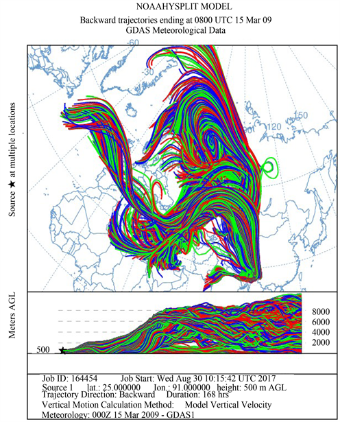


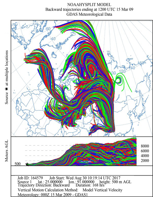
Figure 1. The HYSPLIT air mass back trajectory matrices depicting the transient changes in the atmospheric conditions that lead to the long range transport of pollutant plume to the sampling site in NE India during the sampling in March 2009.
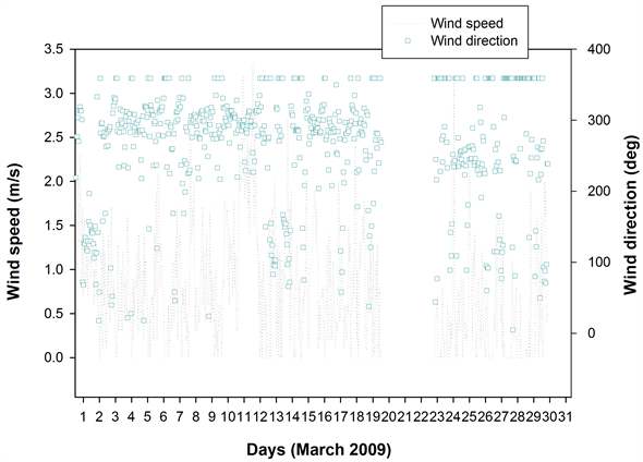
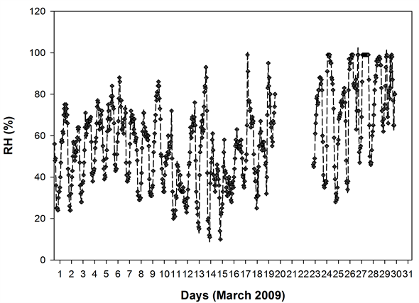
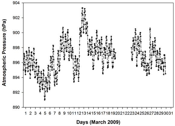
Figure 2. Daily variation of meteorological parameters at the sampling site as measured by the automated weather station.
Anomalous features seen in the S-ratios―the molar ratio of to total SOx ( ), an indicator of the oxidation efficiency of SO2 [7] [9] ―during this plume transport episode is the theme of this paper and a further comparison is made with measurements in January 2010―when no such long range transports prevailed.
Towards this, the sulphate ( ) accumulated in the aerosol samples (PM2.5) collected in periodic intervals were measured on the Dionex Ion Chromatograph. The median SO2 concentrations for the corresponding intervals also were obtained from the time series SO2 data [6] . The S-ratios for the different sampling intervals were then calculated as:
(1)
The median S-ratio for the month is then calculated from the S-ratios for the different intervals.
3.1. and SO2 Variabilities in March 2009: The S-ratio Anomaly
When the transient long range transport brought SO2 plumes to the sampling site, the S-ratios, derived from time series and SO2 measurements, were seen to be unusually low (median value, 0.03). The anomalous SO2 oxidation efficiency patterns can be very well seen in the time series S-ratios for the different sampling intervals (Figure 3), which showed a dip during 11th and 12th March

Figure 3. S-ratios calculated from field measurements, for the different sampling intervals (mean time in Hrs shown along X-axis) in March 2009. The trend seen is a dip in the oxidation efficiency during initial days followed by an increase.
2009 followed by a steady ascend to reach its maximum through to 20th followed by a decrease. The lowest ratio recorded was 0.008 (at 0159 hrs, 12th Mar) and the highest was 0.11 (at 1620 hrs, 20th Mar). Throughout this sampling, the S-ratios remained anomalously low.
Similarly, the measured time series SO2 and (Figure 4) exhibited many unusual features. During 9th, 10th and 11th March, the SO2 variability was governed predominantly by long range transport influx with minimal planetary boundary layer (PBL) height diurnality influence. An interesting observation for these days is that the SO2 and peaks were almost in anti-phase with each other, which may be attributed to the differing mobility pattern and loss mechanisms for SO2 (gas) and (particulate matter), to result in apparent transit time/concentration mismatches in reaching the sampling site.
Observations similar to the one here―viz., ‘the poor correlations/phase-agreements in long range transported air masses’―were reported by [9] when plumes from an accidental oil fire event [31] were detected at their high altitude sampling site Mt. Abu, India, and had then projected the scope for further systematic simulation/field studies on the topic.
From 12th March onwards, the SO2 variability is seen to have a more PBL height diurnality influence. During 12th to 20th also, the SO2 and peaks are in anti-phase, and may be explained by a non-availability of sufficient
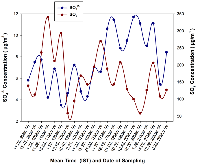
Figure 4. The and SO2 (median) concentrations during each sampling interval (mean time in Hrs shown along X-axis) in March 2009. During the initial days, when SO2 levels were dictated primarily by the long range transport influx, the and SO2 variabilities were almost in anti-phase.
enough OH radicals, which were possibly heavily utilized for the oxidation of large amounts of SO2 [6] and other pollutants [10] in the initial days, to lead to a ‘suppressed oxidation condition’ for the local atmosphere―as evidenced by the anomalously low S-ratios.
During 21st to 26th, when SO2 reduced significantly compared to the initial sampling days, the SO2 and time series variations came in-phase with each other indicating the initiation of a regain of the oxidizing power of the atmosphere via a buildup of sufficient OH.
S-ratio Dependence on SO2 Levels
Figure 5 depicts the S-ratio variabilities as a function of SO2 during the different sampling intervals in March 2009. The ratio is seen to be high at low SO2 concentrations and decreased monotonically with increasing SO2, asymptotically approaching a value of 0.01 at high SO2 concentrations―an observation quite similar to the one reported by [32] . But they reported the S-ratio to asymptotically approach a value of 0.1 at high SO2 concentrations and suggested such a behavior to be consistent with a conversion of about 10% of the fuel sulphur to in the source region followed by (1) oxidation of the SO2 to as the plume transported downwind (2) dilution of the plume with air containing a high fraction of the sulphur present as or (3) a combination of these two processes.
To further explore the notion of ‘suppressed oxidation condition’ over the sampling region and assess the factors contributed to the anomalous low S-
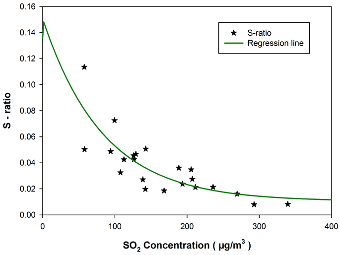
Figure 5. S-ratios plotted as function of SO2 concentration, for samples collected during the plume transport episode in March 2009. The ratios are high at low SO2 concentrations and decreased monotonically with increasing SO2, asymptotically approaching a value of 0.01 at high SO2 concentrations.
ratios, simulation studies with the chemical transport model also were performed, and is detailed below.
3.2. GEOS-Chem Simulation Studies
The GEOS-Chem (v8-03-01) runs were performed with the inventories discussed previously―employing the standard input.geos file―to generate time series SO2 and for the 4˚ × 5˚ grid cell containing the sampling site, and the S-ratios were derived for March 2009. Similar to the experimental observations, the simulations also showed anomalous low S-ratios during 10th to 16th March, and the time series SO2 and variabilities exhibited poor phase agreement (Figure 6).
To study the scenario further, time series OH radicals were generated (Figure 7), from the model by turning ON the ND49 diagnostics. The OH decreased steadily from 7th March 2009 to reach the lowest of the month on 16th, followed by an ascend. Further, the time series OH normalized to time series SO2, referred here as OHspecific gave ‘consistently suppressed values’ during 10th to 16th (Figure 8), thus explaining the observed ‘S-ratio anomaly’ for the period.
Having seen ‘suppressed oxidation conditions’ in both experiments and simulations, it is worth assessing the contributions from factors such as ‘Transport’, ‘dry deposition’ and ‘dust load’ to the scenario. Sensitivity simulations―similar to the ones performed by [9] ―can help resolve some of these factors and are detailed in the following sections 3.2.1 to 3.2.3. From these, the
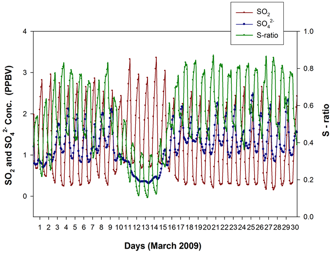
Figure 6. Time series SO2, and S-ratios from GEOS-Chem model for March 2009, for the 4˚ × 5˚ grid cell containing the sampling site. Similar to the experimental observations, the simulations showed anomalous low S-ratios during 10th to 16th, and the SO2 and variabilities exhibited poor phase agreement.

Figure 7. The time series OH radical concentrations from GEOS-Chem model for March 2009 for the 4˚ × 5˚ grid cell containing the sampling site. The OH decreased steadily from 7th to reach the lowest of the month by 16th.
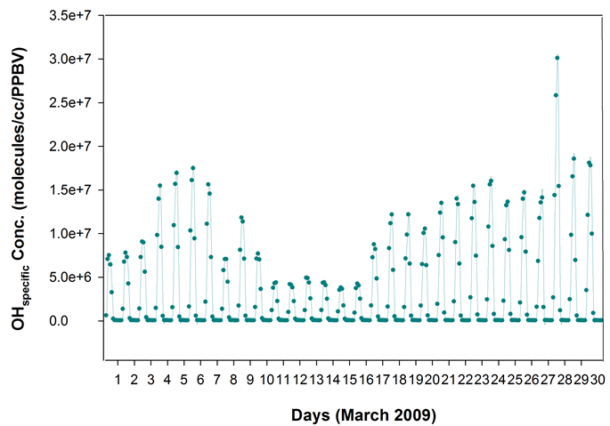
Figure 8. Time series OH (molecules/cc) normalized to time series SO2 (PPBV) from the GEOS-Chem model-referred as OHspecific-for the 4˚ × 5˚ grid cell containing the sampling site, for March 2009. The OHspecific gave ‘consistently suppressed values’ during 10th to 16th.
effect of switching OFF different ‘processes’ on the SO2, , and S-ratios are assessed via the equation:
(2)
where:
ΔSpecies(process) = Percent Difference in Species concentration/value in the absence of the ‘Process’
Species = Species concentration/value from the baseline run employing the standard input.geos file
Species' = Species concentration/value from the sensitivity run with the particular ‘process’ turned OFF
The ‘Species’ mentioned here are SO2, , and S-ratio respectively.
3.2.1. Effect of Transport on the S-ratio Anomaly
To assess the role of transport on the anomalous low S-ratios and poor phase agreements, sensitivity simulations were performed with ‘Transport OFF’. The ‘percent difference in SO2, , and S-ratios in the absence of transport’ (Figure 9) for the GEOS-Chem 4˚ × 5˚ grid cell containing the sampling site, termed ΔSO2(Transport), and ΔS-ratio(Transport) respectively are then obtained via the Equation (2). Here, the ‘process’ in the equation is ‘Transport’.
The ΔSO2(Transport) showed negative values during 3rd to 11th March ’09 with the lowest on 8th (except for a slight increase on 9th). This suggests the prominent ‘long range transported SO2 presence’ over the sampling region during 3rd to 11th, supporting the observations of [6] . It then increased (switched to positive) during 12th to 15th March, possibly suggesting an ‘accumulation’ of long range transported SO2 over the sampling region in the ‘absence of transport’. The also decreased during 3rd to 11th March (except for the slight increase on 9th and 10th) with minimal diurnal fluctuations. The values then increased from 12th March, giving a peak between 12th and 16th―indicating that

Figure 9. ΔSO2(Transport), Δ (Transport), and ΔS-ratio(Transport) from sensitivity simulations, for the GEOS-Chem 4˚ × 5˚ grid cell containing the sampling site. The ΔS-ratio(Transport) showed a major enhancement during 10th to 16th March suggesting that the ‘Transport’ caused significant reductions in the S-ratios (max: 114%, on 13th).
the transport significantly reduced the levels over the sampling region during this period, possibly attributed to the enhanced presence of other pollutants including CO and NOx competing for the available OH and hence reducing the SO2 oxidation rate as will be detailed in Section 3.2.4.―and the enhancements were much more pronounced than that of ΔSO2(Transport). The diurnal fluctuations in during these days were very minimal. The ΔS-ratio(Transport) showed a major enhancement during 10th - 16th March suggesting that the ‘Transport’ caused significant reductions in the S-ratios (max: 114%, on 13th March), during these days due to the enhanced presence of SO2 compared to when ‘Transport is ON’―explained by the OH deficiency, for the high pollutant levels.
The predominant presence of SO2 compared to in the model predictions are similar to the experimental observations and support the arguments of [6] ―viz. the ‘enhanced transport’ of SO2 containing plumes, associated with the cold air outbreak and dust storm events [29] [33] , has contributed to the high SO2 levels. Also this sensitivity simulation supports the notion that ‘ anti-phase in the initial days were governed by the long range transport patterns’ of the two species, with their ‘relative transit-time/loss-mechanism mismatches’ being a prominent factor.
3.2.2. Effect of Dry Deposition on the S-ratio Anomaly
Dry deposition is known to play major roles in the removal of air pollutants from atmosphere [9] [34] - [41] . To study the effect of dry deposition on the poor phase agreements and anomalous low S-ratios, sensitivity simulations were performed with ‘Dry Deposition OFF’. The ‘percent difference in SO2, , and S-ratios in the absence of Dry Deposition’ (Figure 10) for the 4˚ × 5˚ grid cell, termed ΔSO2(DryDeposition), and ΔS-ratio(DryDeposition) respectively, are then obtained via the Equation (2). Here, the ‘process’ in the equation is ‘Dry Deposition’.
The ΔSO2(DryDeposition) gave only positive values throughout March 2009, but with varying magnitudes. During 10th to 15th, it showed very minimal diurnal variation and the dry deposition losses were among the lowest of the month. The gave both positive and negative values. During 3rd to 9th March the values were negative, with the lowest on 3rd and 4th showing the prominent ‘dry deposition’ effects in enhancing the during this period―possibly attributed to the enhanced levels of other pollutant gases in the absence of dry deposition, competing for the available OH and hence reducing its availability for SO2 oxidation. The switched to positive during 11th - 14th March with the peak on 11th and 12th and exhibited minimal diurnal fluctuations. In other words, during these days the ‘dry deposition’ significantly reduced the concentration. The ΔS-ratio(DryDeposition) remained mostly negative throughout March 2009, indicating that the ‘dry deposition’ has been enhancing the S-ratio―as suggested by [8] , that when dry deposition losses are minimized, an enhanced retention time for SO2 can lead to efficient oxidation to .
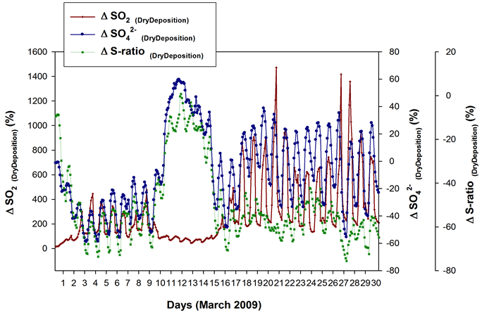
Figure 10. ΔSO2 (DryDeposition), Δ (DryDeposition) and ΔS-ratio (DryDeposition) from sensitivity simulations, for the GEOS-Chem 4˚ × 5˚ grid cell containing the sampling site. The ΔS-ratio(DryDeposition) increased (less negative) during 10th to 14th March with values touching almost zero (on 11th).
During 3rd to 9th March, the S-ratio enhancement due to ‘dry deposition’ is among the highest of the month. The ΔS-ratio(DryDeposition) increased (less negative) during 10th to 14th with values touching almost zero (on 11th March). In other words, during this period the S-ratio enhancements due to ‘dry deposition’ were very minimal. This may be explained as follows. In the absence of dry deposition, the enhanced retention time of SO2 is expected to enhance the formation [8] via the oxidation by OH. But since the OHspecific values for this period is very low the oxidation efficiency is very minimal, and so the enhancement in via the oxidation process is negligible even while the dry deposition is switched OFF.
3.2.3. Effect of Dust Load on the S-ratio Anomaly
The sampling period in March 2009 had witnessed occasional rise in the atmospheric dust load [6] [10] [33] . It is known that reactions with mineral particles influence sulphur budgets downwind dust source regions [9] [42] [43] [44] . In order to assess the ‘dust load’ factor in the OH levels and photochemical activity, sensitivity simulations were performed with ‘dust emission OFF’. The ‘percent difference in SO2, , and S-ratios in the absence of Dust Emission’ (Figure 11), termed ΔSO2(DustEmission), and ΔS-ra- tio(DustEmission) respectively, are then obtained via the equation (2). Here, the ‘process’ is ‘Dust Emission’.
The ΔSO2(DustEmission) mostly gave positive values except for the two negative spikes each on 5th and 6th March. Many positive spikes with diurnal variability were seen during 7th to 12th, with the most prominent one on 10th March, implying that the dust emission has been pulling down the SO2 levels during these
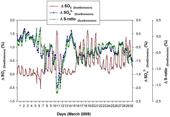
Figure 11. ΔSO2 (DustEmission), Δ (DustEmission) and ΔS-ratio (DustEmission) from sensitivity simulations, for the GEOS-Chem 4˚ × 5˚ grid cell containing the sampling site. ΔS-ratio(DustEmission) mostly gave negative values with the lowest values seen on 10th and 11th March (min. −1.75%) followed by a steady ascend to reach near zero by 14th.
days. During 13th to 15th, the ΔSO2(Dust Emission) again showed minimal spikes (in the positive direction). The showed a prominent negative spike on 7th March. It mostly gave negative values with the lowest (most negative) seen during 10th and 11th―viz., the dust emission helped enhance the levels during these days―followed by a steady ascend to reach near zero values by 14th. The ΔS-ratio(DustEmission) more or less followed the variability pattern. ΔS-ratio(DustEmission) mostly gave negative values with the lowest values seen on 10th and 11th March (min: −1.75%) followed by a steady ascend to reach near zero by 14th. In other words, the ‘dust emission’ enhanced the S-ratios during 10th and 11th, which then reduced to near zero by 14th March.
3.2.4. The Role of CO and NOx on the S-ratio Anomaly
Based on projections from photochemical box model studies [45] - [51] , the various possible scenarios arising out of low/high NOx conditions to the OH availability in a polluted atmosphere are vividly discussed in [2] . They forecast ‘poor OH recycling efficiencies’ to prevail under depleted NOx and elevated CO and CH4 concentrations. On the contrary the system would go autocatalytic at high NOx conditions when the OH recycling is quite efficient, leading to a runaway of oxidants. Also, they projected that the high NOx system leads to unstable conditions and that short periods with high (initially autocatalytic) OH formation were to follow long periods of OH suppression.
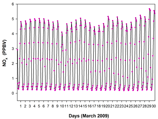
To assess the possible roles by the CO and NOx in the anomalous OH fluctuations―and hence to the poor S-ratios―time series concentrations of these species were obtained from the model along with time series PBL (Figure 12) via
 (a)
(a)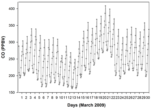 (b)
(b)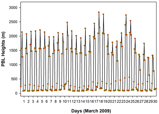 (c)
(c)
Figure 12. The time series NOx, CO and PBL height from GEOS-Chem model, for the 4˚ × 5˚ grid cell containing the sampling site. The NOx showed a dip on 10th March which coincided with the triggering of ‘below threshold OHspecific’, while the CO remained high especially during the few days preceding 10th.
the ND49 diagnostics. The NOx showed a dip on 10th March which coincided with the triggering of ‘below threshold OHspecific’, while the CO remained high especially during the days preceding 10th March (the percentage reduction in the night time CO on 10th March was less significant when compared to those of NOx)―a scenario quite similar to the one mentioned in [2] . The night time dip in NOx and CO on 10th March also coincided with a higher night time PBL on the 10th. The depleted NOx on 10th could have triggered a ‘period of poor OH recycling’ efficiency which when coincided a high SO2 influx from the long range transport, possibly contributed, at least in part, to the ‘period of OH suppression’ and to the anomalous low S-ratios.
3.3. An OH Minimum in NE India and the Neighboring Region
The degree of temporal and spatial variability of tropospheric OH and its effects on the species life time has been a topic of debate [52] - [57] . In the wake of the very limited direct OH radical measurements available for the region, GEOS-Chem model simulations can help provide significant insights into the geographical distribution pattern of OH.
Figure 13 shows the mean OH concentrations for different months of the year 2009, from the GEOS-Chem model. A clear OH minimum is seen over the region surrounding (20˚N, 95˚E) spanning parts of the north-east India and the adjacent regions to the south-east of it. This minimum is prevalent throughout
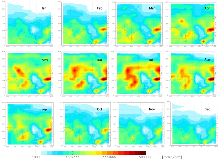
Figure 13. The geographical pattern of the distribution of OH radical for different months of the year 2009, from the GEOS-Chem model. A clear minimum is seen over the region surrounding (20˚N, 95˚E) spanning parts of the north-east India and the adjacent regions to the south-east of it. This minimum is prevalent throughout the year, though the magnitude and the area of influence have a seasonality to it.
the year, though the magnitude and the area of influence have a seasonality to it. This model prediction of an OH minimum can have significant implications to the present understanding on the oxidizing power of the regional atmosphere and hence on the air quality, especially during the long range pollution transport episodes associated with spring time cold air outbreaks. For example, [58] from their model studies showed that an ‘OH minimum’ in west Pacific could reduce the upper free tropospheric aerosol surface area density by up to 25% (due to less efficient conversion of SO2 into sulphate), while that in the lowermost stratosphere increase by more than 5% (due to increased SO2 transport into the stratosphere and conversion into sulphate at higher altitudes).
It is clear that the OH minimum conditions reflected in the model simulations, for the region, could well be the possible explanation for the suppressed S-ratio values during the plume transport episode in March 2009. The ‘OH minimum’ in the model simulations along with the ‘anomalous low S-ratios’ in the field measurements, underlines the impending need for systematic field measurements of OH in north-east India and the adjoining regions―in the wake of the region’s growing anthropogenic emissions.
3.4. , SO2, and S-ratio Variabilities in January 2010
The simultaneous measurements of ambient SO2 and were again performed at our sampling site, in January 2010. This sampling period didn’t see any major long range transports [6] and the air mass back trajectories extended mostly to the Indo-Gangetic plane (figures not shown). For this month, no any kind of anomalies were seen in the SO2 oxidation efficiencies, and the S-ratios (Figure 14) were well within the acceptable limits, with a monthly median value of 0.32. The S-ratio values for this month are comparable to those reported by [9] , for their western Indian site, Mt. Abu. A very good phase-agreement is seen between the SO2 and time series during the different sampling intervals for this month.
This observation of an in-phase varying time series and a monthly median S-ratio value on par with those reported from western India [9] , would possibly imply that under the present local emission conditions of the region, the oxidizing power of the regional atmosphere is still somewhat sufficient to have normal oxidation rates for the trace gases including SO2, which becomes insufficient during major long range pollution transport episodes―peaking in the spring time [6] [10] when cold air outbreaks cause significant pollutant transport from far flung regions.
4. Conclusions
We have reported an instance of ‘suppression in atmospheric SO2 oxidation efficiency’ during a major plume transport episode detected at our sampling site Shillong (25.67˚N, 91.91˚E, 1064 m ASL). Anomalously low S-ratios (median, 0.03) were observed in the field measurements during the episode in March 2009
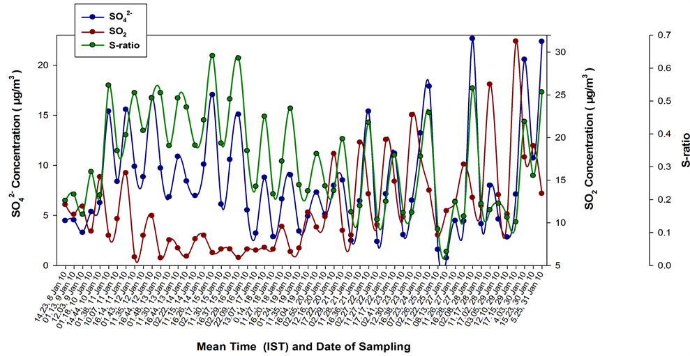
Figure 14. The time series and SO2 (median) concentrations as well as S-ratios during each sampling interval (mean time in Hrs shown along X-axis) for the sampling period in January 2010. The S-ratios for this month were well within the acceptable limits and phase-agreement is seen between the SO2 and variabilities.
and the time series and SO2 exhibited unusual features in the ‘relative phase’ of their peaks. During the initial days, when SO2 levels were dictated primarily by the long range transport influx (viz. high SO2 levels even during the high PBL conditions in daytime), the and SO2 variabilities were almost in anti-phase―which has been attributed to the differing mobility patterns and loss mechanisms for the two species. When SO2 was governed primarily by the PBL effects in the latter days (viz. low (high) SO2 levels during day (night) time when PBL is high (low)), the anti-phase is explained by a ‘depleted OH level’―a major portion of which were possibly consumed in the initial days for the oxidation of large amounts of SO2 and other pollutants.
Simulations employing the GEOS-Chem (v8-03-01) model, also showed suppressed oxidation conditions during 10th to 16th March 2009, with characteristic low S-ratios and poor phase agreements, which are explained by a steadily decreasing OH from 7th to 16th. Further, the OH normalized to SO2, referred as OHspecific, was consistently low during the above days. The contributions from ‘Transport’, ‘Dry Deposition’ and ‘Dust Emission’ to the suppressed oxidizing conditions were also assessed through sensitivity simulations. The ‘Transport’ caused major reductions in the S-ratio (max: 114%, on 13th) during 10th to 16th March. The ‘dust emission’ is seen to boost the S-ratios by up to 1.75% (during 10th and 11th). The time series NOx from the model showed a dip on 10th March which coincided with the triggering of ‘below threshold OHspecific’, while the CO remained high―a scenario which could have possibly helped, at least in part, trigger a ‘poor OH recycling efficiency’. The geographical distribution pattern of OH from the GEOS-Chem model showed a pronounced minimum over the region surrounding (20˚N, 95˚E) spanning parts of northeast India and the adjacent regions to the southeast of it―prevalent throughout the year, though the magnitude and the area of influence have a seasonality to it―with significant implications to reducing the oxidizing power of the regional atmosphere. A second set of SO2 and field measurements during January 2010―when no major long range transports prevailed―showed no any kind of the anomalies of the former sampling month and the S-ratios were well within the acceptable limits, with a monthly median value of 0.32. These observations possibly imply that under the present local emission conditions of the region, the oxidizing power of the regional atmosphere is still somewhat sufficient to have normal oxidation rates for the pollutant gases, while the OH become insufficient during major long range pollution transport episodes―peaking during the spring time when cold air outbreaks cause air mass transport from far flung regions.
Acknowledgements
The ISRO-Geosphere Biosphere Program (Department of Space, Government of India) is gratefully acknowledged for the partial financial support for this study. The authors are highly grateful to Prof. M. M. Sarin, Physical Research Laboratory, India, for the invaluable scientific discussions and support towards this study.
Cite this paper
Francis, T., Kundu, S.S., Rengarajan, R. and Borgohain, A. (2017) SO2 Oxidation Efficiency Patterns during an Episode of Plume Transport over Northeast India: Implications to an OH Minimum. Journal of Environmental Protection, 8, 1119-1143. https://doi.org/10.4236/jep.2017.810071
References
- 1. Levy, H. (1971) Normal Atmosphere: Large Radical and Formaldehyde Concentrations Predicted. Science, 173, 141-143. https://doi.org/10.1126/science.173.3992.141
- 2. Lelieveld, J., Peters, W., Dentener, F.J. and Krol, M.C. (2002) Stability of Tropospheric Hydroxyl Chemistry. Journal of Geophysical Research, 107, 4715. https://doi.org/10.1029/2002JD002272
- 3. McConnell, J.C., McElroy, M.B. and Wofsy, S.C. (1971) Natural Sources of Atmospheric CO. Nature, 233, 187-188. https://doi.org/10.1038/233187a0
- 4. Crutzen, P.J. (1973) A Discussion of the Chemistry of Some Minor Constituents in the Stratosphere and Troposphere. Pure and Applied Geophysics, 106-108, 1385-1399. https://doi.org/10.1007/BF00881092
- 5. Chameides, W. and Walker, J.C.G. (1973) A Photochemical Theory of Tropospheric Ozone. Journal of Geophysical Research, 78, 8751-8760. https://doi.org/10.1029/JC078i036p08751
- 6. Francis, T. (2011) Effect of Asian Dust Storms on the Ambient SO2 Concentration over North-East India: A Case Study. Journal of Environmental Protection, 2, 778-795. https://doi.org/10.4236/jep.2011.26090
- 7. Kaneyasu, N., Ohta, S. and Murao, N. (1995) Seasonal Variation in the Chemical Composition of Atmospheric Aerosols and Gaseous Species in Sapporo, Japan. Atmospheric Environment, 29, 1559-1568. https://doi.org/10.1016/1352-2310(94)00356-P
- 8. Miyakawa, T., Takegawa, N. and Kondo, Y. (2007) Removal of Sulfur Dioxide and Formation of Sulfate Aerosol in Tokyo. Journal of Geophysical Research, 112, D13209. https://doi.org/10.1029/2006JD007896
- 9. Francis, T., Sarin, M.M. and Rengarajan, R. (2016) Atmospheric SO2 Oxidation Efficiency over a Semi-Arid Region: Seasonal Patterns from Observations and GEOS-Chem Model. Atmospheric Environment, 125, 383-395. https://doi.org/10.1016/j.atmosenv.2015.09.021
- 10. Rajput, P., Sarin, M. and Kundu, S.S. (2013) Atmospheric Particulate Matter (PM2.5), EC, OC, {WSOC} and {PAHs} from NE-Himalaya: Abundances and Chemical Characteristics. Atmospheric Pollution Research, 4, 214-221. https://doi.org/10.5094/APR.2013.022
- 11. Igarashi, Y., Sawa, Y., Yoshioka, K., Matsueda, H., Fujii, K. and Dokiya, Y. (2004) Monitoring the SO2 Concentration at the Summit of Mt. Fuji and a Comparison with Other Trace Gases during Winter. Journal of Geophysical Research, 109, D17304. https://doi.org/10.1029/2003JD004428
- 12. Luke, W.T. (1997) Evaluation of a Commercial Pulsed Fluorescence Detector for the Measurement of low-Level SO2 Concentrations during the Gas-Phase Sulfur Intercomparison Experiment. Journal of Geophysical Research, 102, 16255-16265. https://doi.org/10.1029/96JD03347
- 13. Luria, M., Boatman, J.F., Harris, J., Ray, J., Straube, T., Chin, J., Gunter, R.L., Herbert, G., Gerlach, T.M. and Van Valin, C.C. (1992) Atmospheric Sulfur Dioxide at Mauna Loa, Hawaii. Journal of Geophysical Research, 97, 6011-6022. https://doi.org/10.1029/91JD03126
- 14. Rastogi, N. and Sarin, M.M. (2005) Long-Term Characterization of Ionic Species in Aerosols from Urban and High-Altitude Sites in Western India: Role of Mineral Dust and Anthropogenic Sources. Atmospheric Environment, 39, 5541-5554. https://doi.org/10.1016/j.atmosenv.2005.06.011
- 15. Rengarajan, R. and Sarin, M.M. (2004) Atmospheric Deposition Fluxes of 7Be, 210Pb and Chemical Species to the Arabian Sea and Bay Bengal. Indian Journal of Marine Sciences, 33, 56-64.
- 16. Bey, I., Jacob, D.J., Yantosca, R.M., Logan, J.A., Field, B.D., Fiore, A.M., Li, Q., Liu, H.Y., Mickley, L.J. and Schultz, M.G. (2001) Global Modeling of Tropospheric Chemistry with Assimilated Meteorology: Model Description and Evaluation. Journal of Geophysical Research, 106, 23073-23095. https://doi.org/10.1029/2001JD000807
- 17. Park, R.J., Jacob, D.J., Field, B.D., Yantosca, R.M. and Chin, M. (2004) Natural and Transboundary Pollution Influences on Sulfate-Nitrate-Ammonium Aerosols in the United States: Implications for Policy. Journal of Geophysical Research, 109, D15204. https://doi.org/10.1029/2003JD004473
- 18. Wang, J., Jacob, D.J. and Martin, S.T. (2008) Sensitivity of Sulfate Direct Climate forcing to the Hysteresis of Particle Phase Transitions. Journal of Geophysical Research, 113, D11207. https://doi.org/10.1029/2007JD009368
- 19. Fairlie, T.D., Jacob, D.J. and Park, R.J. (2007) The Impact of Transpacific Transport of Mineral Dust in the United States. Atmospheric Environment, 41, 1251-1266. https://doi.org/10.1016/j.atmosenv.2006.09.048
- 20. Chen, D., Wang, Y., McElroy, M.B., He, K., Yantosca, R.M. and Le Sager, P. (2009) Regional CO Pollution and Export in China Simulated by the High-Resolution Nested-Grid GEOS-Chem Model. Atmospheric Chemistry and Physics, 9, 3825-3839. https://doi.org/10.5194/acp-9-3825-2009
- 21. Park, R.J., Jacob, D.J., Kumar, N. and Yantosca, R.M. (2006) Regional Visibility Statistics in the United States: Natural and Transboundary Pollution Influences, and Implications for the Regional Haze Rule. Atmospheric Environment, 40, 5405-5423. https://doi.org/10.1016/j.atmosenv.2006.04.059
- 22. Alexander, B., Park, R.J., Jacob, D.J., Li, Q.B., Yantosca, R.M., Savarino, J., Lee, C.C.W. and Thiemens, M.H. (2005) Sulfate Formation in Sea-Salt Aerosols: Constraints from Oxygen Isotopes. Journal of Geophysical Research, 110, D10307. https://doi.org/10.1029/2004JD005659
- 23. Liu, H., Jacob, D.J., Bey, I. and Yantosca, R.M. (2001) Constraints from 210Pb and 7Be on Wet Deposition and Transport in a Global Three-Dimensional Chemical Tracer Model Driven by Assimilated Meteorological Fields. Journal of Geophysical Research, 106, 12109-12128. https://doi.org/10.1029/2000JD900839
- 24. Wesely, M.L. (1989) Parameterization of Surface Resistances to Gaseous Dry Deposition in Regional-Scale Numerical Models. Atmospheric Environment, 23, 1293-1304. https://doi.org/10.1016/0004-6981(89)90153-4
- 25. Vestreng, V. and Klein, H. (2002) Emission Data Reported to UNECE/EMEP. Quality Assurance and Trend Analysis and Presentation of WebDab, MSC-W Status Report 2002. Norwegian Meteorological Institute, Oslo.
- 26. Kuhns, H., Green, M. and Etyemezian, V. (2003) Big Bend Regional Aerosol and Visibility Observational (BRAVO) Study Emissions Inventory. Desert Research Institute, Las Vegas, Nevada.
- 27. Olivier, J.G.J. and Berdowski, J.J.M. (2001) Global Emissions Sources and Sinks, in the Climate System. In: Berdowski, J., Guicherit, R., Heij, B.J. and Lisse, Eds., The Climate System, A.A. Balkema Publishers/Swets and Zeitlinger Publishers, The Netherlands, 33-78.
- 28. Streets, D.G., Zhang, Q., Wang, L., He, K., Hao, J., Wu, Y., Tang, Y. and Carmichael, G.R. (2006) Revisiting China's CO Emissions after the Transport and Chemical Evolution over the Pacific (TRACE-P) Mission: Synthesis of Inventories, Atmospheric Modeling, and Observations. Journal of Geophysical Research, 111, D14306. https://doi.org/10.1029/2006JD007118
- 29. Li, X. and Song, W. (2009) Dust Storm Detection Based on Modis Data. Conference International Conference on Geo-Spatial Solutions for Emergency Management and the 50th Anniversary of the Chinese Academy of Surveying and Mapping, Beijing, 14-16 September 2009.
- 30. Draxler, R.R. and Hess, G.D. (1998) An Overview of the HYSPLIT_4 Modeling System of Trajectories, Dispersion, and Deposition. Australian Meteorological Magazine, 47, 295-308.
- 31. Francis, T. (2012) Temporal Trends in Ambient SO2 at a High Altitude Site in Semi-Arid Western India: Observations versus Chemical Transport Modeling. Journal of Environmental Protection, 3, 657-680. https://doi.org/10.4236/jep.2012.37079
- 32. Daum, P.H., Al-Sunaid, A., Busness, K.M., Hales, J.M. and Mazurek, M. (1993) Studies of the Kuwait Oil Fire Plume during Midsummer 1991. Journal of Geophysical Research, 98, 16809-16827. https://doi.org/10.1029/93JD01204
- 33. Sharma, A.R., Kharol, S.K. and Badarinath, K.V.S. (2010) An Unusual Dust Event over North-Eastern India and Its Association with Extreme Climatic Conditions—A Study Using Satellite Data. Conference Paper: Aerosols & Clouds: Climate Change Perspectives. IASTABulletin, 2000, 214-217.
- 34. Erisman, J.W., Vermeulen, A., Hensen, A., Flechard, C., Dämmgen, U., Fowler, D. and Tuovinen, J.-P. (2005) Monitoring and Modelling of Biosphere/Atmosphere Exchange of Gases and Aerosols in Europe. Environmental Pollution, 133, 403-413. https://doi.org/10.1016/j.envpol.2004.07.004
- 35. Gupta, A., Kumar, R., Kumari, K.M. and Srivastava, S.S. (2004) Atmospheric Dry Deposition to Leaf Surfaces at a Rural Site of India. Chemosphere, 55, 1097-1107. https://doi.org/10.1016/j.chemosphere.2003.08.035
- 36. Lee, B.-K. and Lee, C.-B. (2004) Development of an Improved Dry and Wet Deposition Collector and the Atmospheric Deposition of {PAHs} onto Ulsan Bay, Korea. Atmospheric Environment, 38, 863-871. https://doi.org/10.1016/j.atmosenv.2003.10.047
- 37. Edwards, P.J., Gregory, J.D. and Allen, H.L. (1999) Seasonal Sulfate Deposition and Export Patterns for a Small Appalachian Watershed. Water, Air, and Soil Pollution, 110, 137-155. https://doi.org/10.1023/A:1005087421791
- 38. Yi, S.-M., Holsen, T.M. and Noll, K.E. (1997) Comparison of Dry Deposition Predicted from Models and Measured with a Water Surface Sampler. Environmental Science & Technology, 31, 272-278. https://doi.org/10.1021/es960410g
- 39. Bidleman, T.F. (1988) Atmospheric Processes. Environmental Science & Technology, 22, 361-367. https://doi.org/10.1021/es00169a002
- 40. Zeller, K., Donev, E., Bojinov, H. and Nikolov, N. (1997) Air Pollution Status of the Bulgarian Govedartsi Ecosystem. Environmental Pollution, 98, 281-289. https://doi.org/10.1016/S0269-7491(97)00144-9
- 41. Raymond, H.A., Yi, S.-M., Moumen, N., Han, Y. and Holsen, T.M. (2004) Quantifying the Dry Deposition of Reactive Nitrogen and Sulfur Containing Species in Remote Areas Using a Surrogate Surface Analysis Approach. Atmospheric Environment, 38, 2687-2697. https://doi.org/10.1016/j.atmosenv.2004.02.011
- 42. Dentener, F.J., Carmichael, G.R., Zhang, Y., Lelieveld, J. and Crutzen, P.J. (1996), Role of Mineral Aerosol as a Reactive Surface in the Global Troposphere. Journal of Geophysical Research, 101, 22869-22889. https://doi.org/10.1029/96JD01818
- 43. Li-Jones, X. and Prospero, J.M. (1998) Variations in the Size Distribution of Non-Sea-Salt Sulfate Aerosol in the Marine Boundary Layer at Barbados: Impact of African Dust. Journal of Geophysical Research, 103, 16073-16084. https://doi.org/10.1029/98JD00883
- 44. Zhang, Y. and Carmichael, G.R. (1999) The Role of Mineral Aerosol in Tropospheric Chemistry in East Asia—A Model Study. Journal of Applied Meteorology, 38, 353-366. https://doi.org/10.1175/1520-0450(1999)038<0353:TROMAI>2.0.CO;2
- 45. Guthrie, P.D. (1989) The CH4-CO-OH Conundrum: A Simple Analytic Approach. Global Biogeochemical Cycles, 3, 287-298. https://doi.org/10.1029/GB003i004p00287
- 46. Kleinman, L.I. (1994) Low and High NOx Tropospheric Photochemistry. Journal of Geophysical Research, 99, 16831-16838. https://doi.org/10.1029/94JD01028
- 47. Prather, M.J. (1994) Lifetimes and Eigenstates in Atmospheric Chemistry. Geophysical Research Letters, 21, 801-804. https://doi.org/10.1029/94GL00840
- 48. Stewart, R.W. (1995) Dynamics of the Low to High NOx Transition in a Simplified Tropospheric Photochemical Model. Journal of Geophysical Research, 100, 8929-8943. https://doi.org/10.1029/95JD00691
- 49. Krol, M.C. and Poppe, D. (1998) Nonlinear Dynamics in Atmospheric Chemistry Rate Equations. Journal of Atmospheric Chemistry, 29, 1-16. https://doi.org/10.1023/A:1005843430146
- 50. Poppe, D. and Lustfeld, H. (1996) Nonlinearities in the Gas Phase Chemistry of the Troposphere: Oscillating Concentrations in a Simplified Mechanism. Journal of Geophysical Research, 101, 14373-14380. https://doi.org/10.1029/96JD00339
- 51. Hess, P.G. and Madronich, S. (1997) On Tropospheric Chemical Oscillations. Journal of Geophysical Research, 102, 15949-15965. https://doi.org/10.1029/97JD00526
- 52. Hanisco, T.F., Lanzendorf, E.J., Wennberg, P.O., Perkins, K.K., Stimpfle, R.M., Voss, P.B. and Midwinter, C. (2001) Sources, Sinks, and the Distribution of OH in the Lower Stratosphere. The Journal of Physical Chemistry A, 105, 1543-1553. https://doi.org/10.1021/jp002334g
- 53. Lelieveld, J., Dentener, F.J., Peters, W. and Krol, M.C. (2004) On the Role of Hydroxyl Radicals in the Self-Cleansing Capacity of the Troposphere, Atmos. Chemical Physics, 4, 2337-2344.
- 54. Berglen, T.F., Berntsen, T.K., Isaksen, I.S.A. and Sundet, J.K. (2004) A Global Model of the Coupled Sulfur/Oxidant Chemistry in the Troposphere: The Sulfur Cycle. Journal of Geophysical Research, 109, D19310. https://doi.org/10.1029/2003JD003948
- 55. Manning, M.R., Lowe, D.C., Moss, R.C., Bodeker, G.E. and Allan, W. (2005) Short-Term Variations in the Oxidizing Power of the Atmosphere. Nature, 436, 1001-1004. https://doi.org/10.1038/nature03900
- 56. Rohrer, F. and Berresheim, H. (2006) Strong Correlation between Levels of Tropospheric Hydroxyl Radicals and Solar Ultraviolet Radiation. Nature, 442, 184-187. https://doi.org/10.1038/nature04924
- 57. Montzka, S.A., Krol, M., Dlugokencky, E., Hall, B., Jöckel, P. and Lelieveld, J. (2011) Small Interannual Variability of Global Atmospheric Hydroxyl. Science, 331, 67-69. https://doi.org/10.1126/science.1197640
- 58. Rex, M., Wohltmann, I., Ridder, T., Lehmann, R., Rosenlof, K., Wennberg, P., Weisenstein, D., Notholt, J., Krüger, K., Mohr, V. and Tegtmeier, S. (2014) A Tropical West Pacific OH Minimum and Implications for Stratospheric Composition. Atmospheric Chemistry and Physics, 14, 4827-4841. https://doi.org/10.5194/acp-14-4827-2014