Communications and Network
Vol.08 No.01(2016), Article ID:64014,11 pages
10.4236/cn.2016.81006
Performance Comparison of a QoS Aware Routing Protocol for Wireless Sensor Networks
Bhaskar Bhuyan1, Nityananda Sarma2
1Department of IT, Sikkim Manipal Institute of Technology, Rangpo, India
2Department of Computer Science and Engineering, Tezpur University, Napaam, India

Copyright © 2016 by authors and Scientific Research Publishing Inc.
This work is licensed under the Creative Commons Attribution International License (CC BY).
http://creativecommons.org/licenses/by/4.0/


Received 18 December 2015; accepted 26 February 2016; published 29 February 2016
ABSTRACT
Quality of Service (QoS) in Wireless Sensor Networks (WSNs) is a challenging area of research because of the limited availability of resources in WSNs. The resources in WSNs are processing power, memory, bandwidth, energy, communication capacity, etc. Delay is an important QoS parameter for delivery of delay sensitive data in a time constraint sensor network environment. In this paper, an extended version of a delay aware routing protocol for WSNs is presented along with its performance comparison with different deployment scenarios of sensor nodes, taking IEEE802.15.4 as the underlying MAC protocol. The performance evaluation of the protocol is done by simulation using ns-2 simulator.
Keywords:
Wireless Sensor Networks, Quality of Service, Delay, Time Constraint

1. Introduction
WSNs are collection of large number of sensor nodes deployed for sensing and gathering data [1] . This gathered data are sent to a control station called sink or base station for further processing. Different applications in which WSNs can be deployed are environment sensing, health care, surveillance, industrial control, home automation, security services, etc. [2] . A simple wireless sensor network model is shown in Figure 1, redrawn from [3] .
Provisioning of Quality of Service (QoS) in WSNs is challenging task. End to end delay is considered to be one of the important QoS parameter in WSNs for delivery of certain time critical information to the Sink or Base Station within a specific deadline. Some examples of such applications are military surveillance, industrial
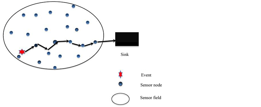
Figure 1. A typical wireless sensor network.
monitoring, healthcare, disaster management, etc. Like end to end delay, some of the other QoS parameters in WSNs are reliability, energy, data accuracy, coverage, etc.
MAC protocol plays an important role for accessing the communication medium. Although different MAC protocols are used in sensor networks, IEEE802.15.4 is the de facto standard and it can be used under the scopes of different research objectives such as minimization of power consumption, improving packet delivery ratio, improving channel utilization, reducing end to end delay, etc. [4] . IEEE802.15.4 specifies the physical and MAC sublayer for low rate personal area networks [5] .
In this paper an extended version of our earlier work [3] is presented along with inclusion of a module for deadline estimation. The work presented in [3] is a preliminary version of the work presented in this paper. The deadline estimation module can be used for making an estimation of deadline when certain sensing information is to be sent to the sink within a time constraint for random deployment of sensor nodes. A detail working principle of the protocol is presented focusing mainly on the packet forwarding scheme. We have also extended our work for performance comparison with different scenarios considering grid and random deployment of sensor nodes and taking IEEE802.15.4 as the underlying MAC protocol. Various simulation scenarios are created by varying the number of sensor nodes and simulation time for both the deployment scenarios. Different performance metrics such as end to end delay, packet delivery ratio, deadline miss ratio, etc. are measured by simulation.
The rest of this paper is organized as follows. In Section 2, we have presented a review of some of the existing related works and discussed their pros and cons. In Section 3, we have presented the working principle of the protocol along with the deadline estimation module. Section 4 presents the performance analysis of the protocol considering different simulations scenarios and finally Section 5 concludes the paper.
2. Related Works
Numerous literatures are available in the area of wireless sensor networks. Provisioning of QoS in wireless sensor networks is an emerging field of research. In this section a brief review of some of the existing QoS aware routing protocols has been presented mainly focusing on delay awareness and reliability of the routing protocols in wireless sensor networks.
SPEED [6] is a stateless real-time communication protocol in WSNs proposed by T. He et al. This protocol meets the end to end delay requirement by uniform communication speed in every hop in the network by feedback control mechanism and non-deterministic QoS aware geographic-forwarding. The limitation of SPEED protocol is that it treats both real time and non real time packets equally. It also suffers from low reliability. More over the protocol is not energy aware.
Akkaya et al. proposed an energy aware QoS routing protocol in wireless sensor networks [7] , which try to find energy efficient paths along which required end to end delay can be fulfilled. Each node classifies the incoming packets and forwards the real time and non real time packets to different priority queues. The delay requirement is converted into bandwidth requirement. The use of class based priority queuing is complicated mechanism and costly for resource constraint sensor nodes.
MMSPEED [8] is an extension of the SPEED proposed by E. Felemban et al. This protocol supports multiple communication speeds over multipath and provides differentiated reliability. This protocol is provides probabilistic QoS differentiation with respect to timeliness and reliability domains. The limitation with MMSPEED is that it does not take energy into consideration while routing the packets.
RAP [9] is a velocity based Real-time Architecture and Protocol proposed by Chenyang Lu et al. Here the required velocity is calculated based on deadline and destination of packets. Priorities of packets are assigned in the velocity-monotonic order in such a way that a high velocity packet is forwarded earlier than a lower velocity packet.
RPAR [10] is a Real time Power-aware Routing in wireless sensor networks proposed by O. Chipara et al. This protocol achieves application specific packet transmission delay with lower energy consumption by dynamically adjusting the transmission power of the sensor nodes while taking routing decisions. This protocol is subject to frequent network topology changes because of dynamic adjustment of transmission power. The limitation of this protocol is that it does not optimize the network life time.
MCMP [11] is a Multi Constrained QoS Multi Path routing protocol in wireless sensor networks proposed by X. Huang and Y. Fang. This protocol is based on certain QoS requirements such as delay and reliability. Here an optimization problem for end to end delay is formulated and solved by linear programming. Packets are transmitted by multiple paths with moderate energy expenditure. The protocol prefers to route information through paths having minimum number of hops for fulfillment of QoS requirement.
Z. Lei et al. proposed FT-SPEED [12] , which is an extension of SPEED protocol. This protocol takes care of routing holes while transmitting packets to its destination. Path lengths become longer due to routing holes and as a result packets may not be delivered to its sink before its deadline.
Our routing protocol presented in this paper attempts to provide QoS in delay aware applications of WSNs mainly considering delay and reliability as the QoS parameters. Although, all the works mentioned above attempts to provide QoS, however many of them are not energy aware. In our work, the routing protocol takes energy also into consideration while forwarding the packets to the sink.
3. Delay Aware Routing Protocol
This is an extended version of our earlier work [3] with the inclusion of a new module for deadline estimation. The deadline estimation module can be used for estimating a deadline for scenarios when sensor nodes are deployed randomly. We have also extended our work by giving a detail operation of the packet forwarding scheme. A detail working principle of the protocol with the newly included module for deadline estimation is presented below.
3.1. Assumptions
We have assumed that sensor nodes are homogeneous in nature. The Sink is GPS enabled and broadcast its location information to all sensor nodes. Each sensor node knows its location by some localization techniques as in [13] . All sensor nodes are static in nature having very less mobility. Initial energy level and radio range of all sensor nodes are equal.
3.2. Operation of the Protocol
The main functionality of the protocol is divided into three parts as mentioned below:
1) Network Configuration and Neighborhood Management.
2) Deadline Estimation.
3) Data Forwarding.
3.2.1. Network Configuration and Neighborhood Management
Initially each sensor nodes explore its one hop neighbors by exchanging a HELLO and ACK control packets. The format of the HELLO packet and ACK packets are shown in Figure 2(a) and Figure 2(b) respectively. The value of the packet type field can be 0 or 1 (0 for HELLO and 1 for ACK). This neighbor discovery information
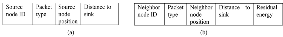
Figure 2. (a) Format of HELLO and (b) ACK control packets.
is stored in each sensor node in the form of a table. This table is updated periodically.
After neighbor discovery phase each sensor node broadcast an echo packet to its neighboring nodes and records the round trip time of the echo packets for computation of link delay [3] . The computation of link delay for a pair of node (ni, nj) is shown in Equation (1).
 [3] (1)
where:
 : Link delay between node ni and nj.
DelayMAC: Channel access delay.
Delayqueue: Queuing delay.
Delaytx: Transmission delay.
 : Transmission count.
Based on the variation of traffic load on the link, delay may vary in the link. After link delay computation each sensor node maintains a data forwarding table based on the information in the neighbor discovery table and estimated link delay. This data forwarding table is looked up for routing data packets to the sink. The structure of data forwarding table is shown in Table 1.
3.2.2. Deadline Estimation
The density and the number of deployed nodes in wireless sensor networks play an important role for estimation of deadline. For estimating deadline we have adopted the idea from [14] . The sensor nodes are deployed randomly according to poison process [15] . Let distance between a source and the sink is D and the radio range of a sensor node is R. It is assumed that sensor nodes are randomly deployed with density ρ per square meter.
Equation (2) is showing the probability of deploying number of sensor nodes, (M(q) = m) in q square meter
 [14] (2)
The expected number of sensor nodes,  , is a product of ρ and q as shown in Equation (3).
 [14] (3)
The area between the source node and the sink is divided into some small fixed size regions which satisfies the following constraints:
1) Each region has at least one sensor node.
2) The maximum distance between sensor nodes in two adjoining regions is equal to radio range R.
So the equivalent length of the diagonal of two adjoining region is R as shown in Figure 3, which is redrawn from [14] .
The area of the region is computed as , where
 .
.
Considering the deployment of sensor nodes according to poison process, the expected number of nodes in a region is
 [14] (4)
Here the density, ρ, and the radio range, R, are constant. The value of minimum θ satisfying condition 1) stated above can be computed as below

Table 1. Structure of data forwarding table.
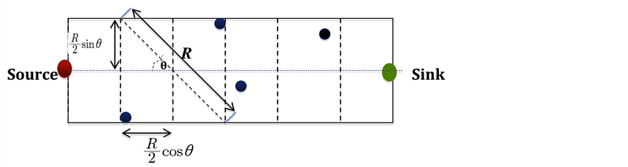
Figure 3. Random deployment of sensor nodes [14] .

 [14] (5)
From Figure 3, the width of a region is computed as  and the expected number of regions from
source to the sink is

So, the expected number of hops from source to the sink is
 [14] (6)
Therefore, the expected delay to the sink can be estimated by the product of number of hops,  , and the average delay of a single hop communication.
3.2.3. Packet Forwarding
A sensor node can play the role of a source node or a forwarding node. If the sink is in the range of the source node or the forwarding node then the packets can be sent directly to the sink. Otherwise packet is forwarded to the sink through multi hop communication. The sensor node looks up its forwarding table and selects one of its neighbor nodes as a forwarding node and sends the data packet to it. The format of a data packet is shown in Figure 4.
The steps of the packet forwarding scheme is summarized below.
1) A sensor node, S, senses the occurrence of an event or a data packet arrives to it.
2) If the Sink, T, is in the transmission range of S then send the data packet to the sink directly.
3) Else S forwards the data packet to a neighbor node which fulfills the conditions stated below.
a) The neighbor node is the most closest neighbor to the sink w.r.t. other neighboring nodes.
b) Propagation speed, Velprov, of data packets provided on the selected link should be greater than or equal to the required propagation speed Velreq on that link.
c) Residual energy of the neighbor node is greater than or equal to threshold energy.
4) If none of the neighboring nodes fulfils conditions 3a), 3b) and 3c) together, then S will look for a neighbor node which is the most closest to the sink and satisfies condition either 3b) or 3c).
In that case a copy of the data packet will also be sent to an alternative neighbor node which is the second most closest neighbor to the sink and fulfills conditions 3b) and 3c).
A typical data forwarding scenario is shown in Figure 5.
The required propagation speed in a link depends on the deadline. The deadline may be specified by the user or estimated by the source node of the event area. In Figure 5, ni is a forwarding node of the source S. Similarly, nj is a forwarding node for the node ni, where i ≠ j. Let d(ni, nj) represents the distance between node ni and nj. The source node S calculates the required end-to-end propagation speed Velreq to the sink T, as Velreq = d(S,T)/tset with respect to the estimated deadline tset. It selects one of its neighbor node as a forwarding node if the provided propagation speed Velprov, of data packets on that link (i.e. source and the neighbor node) is greater than or equal to the required propagation speed Velreq along with the fulfillment of other conditions as stated above. In the process of sending the packet from source to sink every forwarding node computes the required and provided propagation speeds as shown below.
Let,
tset: Estimated deadline for the data packets at source node.
tl: Time left to meet deadline. At the source node, S, tl, is equal to tset and in every forwarding node tl is updated.
If ni is a forwarding node of the source node S in a path between source and the sink then tl at node ni is updated as . A typical scenario for computation of required and offered propagation speed is shown in Figure 6.
The propagation speed provided on a link connecting source node S and node ni is computed in Equation (7).

Figure 4. Format of a data packet.
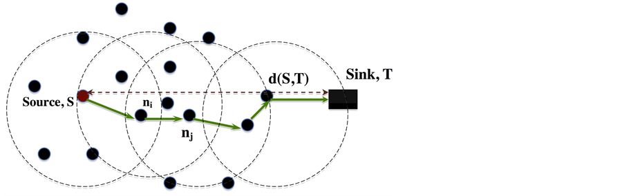
Figure 5. A typical packet forwarding scenario.
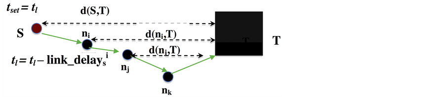
Figure 6. A typical scenario for computation of required and provided propagation speed.
 (7)
(7)
The required propagation speed for the path from node ni to sink T is recomputed at node ni as shown in Equation (8).
 (8)
(8)
The computations shown above are repeated at each forwarding node between source and the sink till the packet reaches the sink.
4. Performance Evaluation
We have evaluated our protocol by simulation using network simulator ns-2 [16] for measuring different performance metrics such as end to end delay, packet delivery ratio, dead line miss ratio etc. Sensor Nodes are deployed randomly in a flat area of 600 × 600 square meters. We have also considered grid deployment of sensor nodes with the same area for the performance comparisons of the protocol. Different simulation scenarios are created by varying the number of sensor nodes as 50, 75, 100, 125, and 150. The simulation time is also varied as 100 seconds, 200 seconds, 300 seconds, 400 seconds and 500 seconds. In our simulation IEEE802.15.4 is used as the underlying MAC protocol. The various simulation parameters chosen are summarized in Table 2.
The performance of our protocol is compared considering the following performance metrics with respect to different scenarios.
1) End to End Delay vs Simulation Time.
2) Packet Delivery Ratio vs Simulation Time.
3) Deadline Miss Ratio vs Number of nodes.
4) Deadline Miss Ratio vs Packet Interval.
5) End to End delay vs Packet Interval.
4.1. End to End Delay vs Simulation Time
End to end delay can be defined as the average end to end delay for all successfully received packets from its source to destination. The average end to end delay is measured for five different scenarios by varying the number of deployed nodes as 50, 75, 100, 125 and 150. For each scenario simulation time is varied as 100 seconds, 200 seconds, 300 seconds, 400 seconds and 500 seconds. Figure 7 shows the average end to end delay for different number of nodes with respect to simulation time for grid and random deployment of sensor nodes.
It is observed that end to delay decreases with increase of simulation time for both grid and random deployment of sensor nodes. For grid deployment, we can see that end to end delay is decreasing uniformly with the
Table 2. Simulation parameters.
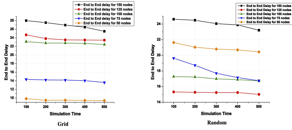
Figure 7. End to end delay (milliseconds) vs simulation time (seconds) for grid and random deployment.
number of nodes. However in case of random deployment this behavior is not strictly followed. This is due to non uniform distances among the sensor nodes in random deployment and because of varying density of nodes distance between source and sink is not uniform for different deployment scenarios of sensor nodes.
4.2. Packet Delivery Ratio vs Simulation Time
Packet Delivery Ratio (PDR) is measured as the ratio of total number of packets received to the number of packet sent without considering the deadline. We have evaluated this performance metric for reliability purpose. Here also Packet Delivery Ratio is measured for five different scenarios by varying the number of deployed nodes as 50, 75, 100, 125 and 150. For each set up simulation time is varied as 100 seconds, 200 seconds, 300 seconds, 400 seconds and 500 seconds as mentioned earlier. We have measured Packet Delivery Ratio for both grid and random deployment. Figure 8 shows the Packet Delivery Ratio for different number of nodes with respect to varying simulation time. It is observed from these experiments that Packet Delivery Ratio increases with the increase of simulation time for both grid and random deployment of nodes. For grid deployment Packet Delivery Ratio is highest for 50 nodes and lowest for 150 nodes. However, for random deployment this pattern is not strictly followed due to non uniform deployment of sensor nodes.
4.3. Deadline Miss Ratio vs Number of Nodes
Deadline Miss Ratio (DMR) is measured as the fraction of packets that missed their deadline. It can be expressed as:

Deadline Miss Ratio is computed to evaluate the performance of the packet forwarding scheme. Figure 9 shows the deadline miss ratio with respect to varying number of sensor nodes for grid and random deployment of sensor nodes. In this experiment the simulation time is fixed at 500 seconds and deadline is set to 19 milli seconds. Each source transmits a packet in the interval of 1 second. It is observed from the graph that number of packets that fails to meet deadline is more with the increase of number of nodes in the network. This behavior is clearly observed for grid deployment of sensor nodes. However, in case of random deployment this behavior is not strictly followed due to non-uniform deployment pattern.
4.4. Deadline Miss Ratio vs Packet Interval
We have also measured Deadline Miss Ratio changing the packet interval time. Packets are generated in the
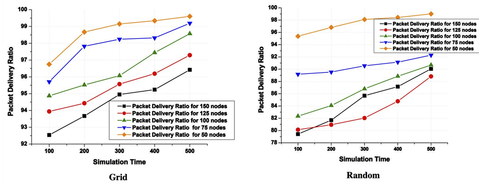
Figure 8. Packet delivery ratio vs simulation time (seconds) for grid and random deployment.
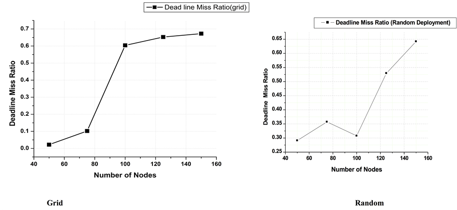
Figure 9. Deadline miss ratio vs number of nodes for grid and random deployment.
intervals of 1 second, 2 seconds, 3 seconds, 4 seconds and 5 seconds. The number of sensor nodes varied as 50, 100 and 150. Here also deadline is 19 milli seconds and simulation time is 500 seconds. It is observed from the graphs shown in Figure 10 that Deadline Miss Ratio decreases with respect to increase of packet interval for both grid and random deployment of sensor nodes.
4.5. End to End Delay vs Packet Interval
Figure 11 is showing the performance of the protocol measured for average end to end delay against packet interval. This experiment is conducted considering the same simulation parameters as mentioned in previous experiment. It has been observed that end to end delay decreases with increase of packet interval time for both grid and random deployment of nodes. This is due to the same reason as mentioned in the previous case, with increase of packet interval there will be lesser congestion in the network and delay incurred by packets will be reduced.
5. Conclusion
In this paper, an extended version of a delay aware routing protocol for wireless sensor networks is presented
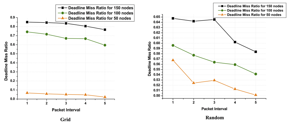
Figure 10. Dead line miss ratio vs packet interval (seconds) for grid and random deployment.
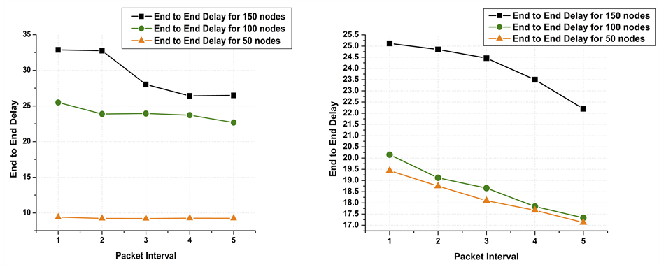
Figure 11. End to end delay (milliseconds) vs packet interval (seconds) for grid and random deployment.
focusing on its performance comparison between grid and random deployment of sensor nodes. The protocol is evaluated using ns-2 simulator by varying the number of sensor nodes from 50 to 150 nodes deployed in a flat area. The various performance parameters considered are end to end delay, packet delivery ratio, deadline miss ratio, etc. From the simulation results, it has been observed that the basic behavior of the protocol is almost similar for both the deployment scenarios. However, we have observed some irregularities in case of random deployment while evaluating the performance parameters such as end to end delay, packer delivery ratio and deadline miss ratio. It has been also observed that in some cases random deployment gives better results in comparison to grid deployment. As a future work, the performance of the protocol can be compared to some of its related protocol.
Cite this paper
BhaskarBhuyan,NityanandaSarma, (2016) Performance Comparison of a QoS Aware Routing Protocol for Wireless Sensor Networks. Communications and Network,08,45-55. doi: 10.4236/cn.2016.81006
References
- 1. Akyildiz, I.F., Su, W., Sankarasubramaniam, Y. and Cayirci, E. (2002) Wireless Sensor Networks: A Survey. Computer Networks, 38, 393-422.
http://dx.doi.org/10.1016/S1389-1286(01)00302-4 - 2. Chen, D. and Varshney, P.K. (2004) QoS Support in Wireless Sensor Network: A Survey. Proceeding of the 2004 International Conference on Wireless Networks (ICWN2004), Las Vegas, June 2004, 227-233.
- 3. Bhuyan, B. and Sarma, N. (2014) A Delay Aware Routing Protocol for Wireless Sensor Networks. International Journal of Computer Science Issues, 11, 60-65.
- 4. Khanafer, M., Guennoun, M. and Mouftah, T., H. (2014) A survey of Beacon-Enabled IEEE 802.15.4 MAC Protocols in Wireless Sensor Networks. IEEE Communication Surveys and Tutorials, 16, 856-876.
http://dx.doi.org/10.1109/SURV.2013.112613.00094 - 5. (2012) IEEE Std 802.14.3-2006, September, Part 15.4: Wireless Medium Access Control (MAC) and Physical Layer (PHY) Specifications for Low-Rate Wireless Personal Area Networks (WPANs).
http://www.ieee.org/Standards - 6. He, T., Stankovic, J.A., Lu, C.Y. and Abdelzaher, T. (2003) SPEED: A Stateless Protocol for Real-Time Communication in Sensor Networks. Proceedings of International Conference on Distributed Computing Systems, Providence, 19-22 May 2003, 46-55.
- 7. Akkaya, K. and Younis, M. (2003) An Energy-Aware QoS Routing Protocol for Wireless Sensor Networks. Proceedings of the IEEE Workshop on Mobile and Wireless Networks (MWN 2003), Providence, May 2003, 20 p.
- 8. Felemban, E., Lee, C. and Ekici, E. (2006) MMSPEED: Multipath Multi-SPEED Protocol for QoS Guarantee of Reliability and Timeliness in Wireless Sensor Networks. IEEE Transaction on Mobile Computing, 5, 736-754.
http://dx.doi.org/10.1109/tmc.2006.79 - 9. Lu, C., Blum, B.M., Abdelzaher, F.T., Stankovic, A.J. and He, T. (2002) RAP: A Real-Time Communication Architecture for Large-Scale Wireless Sensor Network., Proceeding of the Eight IEEE Real-Time and Embedded Technology and Applications Symposium, California, 25-27 September 2002, 55-62
- 10. Chipara, O., He, Z., Ging, G., Chen, Q. and Wang, X. (2006) RPAR: Real-Time Power-Aware Routing in Sensor Networks. Proceeding of 14th International Workshop of QoS, IWQoS, New Haven, 19-21 June 2006, 83-92.
- 11. Huang, X and Fang, Y. (2008) Multi Constrained QoS Multipath Routing Protocol in Wireless Sensor Networks. Wireless Networks, 14, 465-478.
http://dx.doi.org/10.1007/s11276-006-0731-9 - 12. Zhao, L., Kan, B.Q., Xu, Y.J. and Li, X.W. (2007) FT-SPEED: A Fault-Tolerant, Real-Time Routing Protocol for Wireless Sensor Networks. Proceeding of International Conference on Wireless Communications, Networking and Mobile Computing, Shanghai, 21-23 September 2007, 2531-2534.
http://dx.doi.org/10.1109/wicom.2007.630 - 13. Zou, L., Mi, L. and Xiong, Z. (2005) A Distributed Algorithm for the Dead End Problem of Location Based Routing in Sensor Networks. IEEE Transaction on Vehicular Technology, 54, 1509-1522.
http://dx.doi.org/10.1109/TVT.2005.851327 - 14. Heo, J., Hong, J. and Cho, Y. (2009) EARQ: Energy Aware Routing for Real-Time and Reliable Communication in Wireless Industrial Sensor Networks. IEEE Transaction on Industrial Information, 5, 3-11.
http://dx.doi.org/10.1109/TII.2008.2011052 - 15. Ross, M.S. (1983) Stochastic Process. Wiley, New York.
- 16. The Network Simulator, ns-2.
http://www.isi.edu/nsnam/ns/index.html