Communications and Network
Vol.3 No.3(2011), Article ID:6770,7 pages DOI:10.4236/cn.2011.33020
Usage of Erlang Formula in IP Networks
Institute of Telecommunications, Faculty of Electrical Engineering and Information Technology, Slovak University of Technology, Bratislava, Slovak Republic
E-mail: {chromy, kovaci, kavacky}@ut.fei.stuba.sk, suran.jan@pivopraha.cz
Received May 29, 2011; revised July 5, 2011; accepted July 12, 2011
Keywords: Erlang Formula, QoS, VBR Video
Abstract
This paper is concerning of Erlang formulas practical approval and their usage with video flow transfer in IP networks. Erlang formulas were simulated in MATLAB program. Practical verification was realized in defined environment by using of designed video source. The result is comparison of loss calculated by MATLAB and loss of real video data transfer.
1. Introduction
IP networks were not designed for providing multimedia services at the beginning. These networks were intended for data transfer without predefined paths so that in case of breakdown of one of the routers, other path could be chosen [1]. Path of packet can change and so can change transfer parameters.
If we want to use IP networks for voice, video and multimedia transmission, we have to define transfer parameters. These parameters are covered under QoS (Quality of Service). For observance of QoS [2-5] parameters it is necessary to estimate network performance under load and link overflow.
This problem is handled by theory of queuing systems. Therefore we will use Erlang B and Erlang C formulas. Erlang B formula deals with data loss in relation with network load. Erlang C formula defines probability of inserting data into waiting queues and so resembles to IP network behavior, where data queuing occurs before sending further.
1.1. QoS in IP Networks
Increasing number of user requests for application and multimedia services was an impulse for development of protocols that can assure QoS within IP network. This way of requirements has risen not only for network functionality, but also for transfer parameters observance. If these QoS parameter requirements are observed, IP network can even out ISDN (Integrated Services Digital Network) or ATM (Asynchronous Transfer Mode) networks that have bandwidth, delay and availability guaranteed.
Most important parameters are:
• Availability—service reliability during whole connection time.
• Delay—packet transfer time between two reference points.
• Jitter—represents changes in delay.
• Throughput—data transferred per time unit.
• Packet loss—allowed packet loss tolerance per time unit.
QoS assurance in IP network is done through SLA (Service Level Agreement). It is a contract between end user and network provider. SLA includes assurance of many parameters, for example:
• Availability.
• Class of service providing.
• QoS guarantee.
1.2. VBR Video
Because video is basically only a slideshow of pictures displayed at sufficient frequency, it is necessary to compress video flow. Common video flow has a frame rate of 23-30 frames per second [6]. Different lossmaking and also lossless methods are used for each frame. However, compression of individual frames is not a final solution.
CBR (Constant Bit Rate) is a method of saving frames only in compressed form. This data flow does not change its bandwidth requirements, because same type of compression is applied to every frame. With this type of video flow we always have complete picture available and there is no need to use methods for combining more pictures together.
VBR (Variable Bit Rate)—this special data flow uses several type of frames. Position of frame in the video plays important role and it uses differences between pictures. This video flow does not produce data flow of constant bandwidth (it changes in relation to frame differences). This flow can consist of these types of frames:
• Information frame (key frame)—CBR consists only from these frames.
• Prediction frame.
• Differential frame.
1.3. Waiting Queue Systems
WQS (waiting queue systems) are systems with input requirements, service times, queues and other system properties [7-9]. Basic properties of WQS are defined as follows:
 (1)
(1)
where these symbols mean following:
• A – arrival process:
♦ M – poisson distribution
♦ Ek – Erlang distribution
♦ D – deterministic distribution
♦ G – any empirical distribution.
• B –service time distribution.
• X – number of parallel service channels.
• Y – maximum number of requests in source
• Z – maximum queue length.
• V – type of queuing.
WQS are also divided into types with and without feedback. Systems with feedback are called closed systems, when request is returned back. If only part of the service requests is returned back, these systems are hybrid systems. These hybrid types are mostly used in praxis.
2. Simulation Environment
Linux is an open-source operating system (OS). It has gained a lot of fans mostly because of its low system requirements, wide modularity and openness. In this system every part of the core is documented and available [10-13]. Thanks to this attribute, OS Linux or its core is implemented in many devices (routers). In our case we used linux distribution Debian 4.0, installed it on a PC that serves as a router, web server, file server and other applications server. There will also be installed a simulation program for traffic simulation, that will send video flows of defined parameters. Linux is capable of packet modification from its core and we will use this feature. Labeled packets of video flow then will be concentrated into one link or divided. We will install a custom package for traffic engineering, where classes, queues and filters can be created. These three main elements are defining routing mechanisms in router. This type of server with OS linux installed can be a low price alternative to routers used in commercial networks.
2.1. IP Tables
IP tables is a mechanism implemented directly into core of Linux operating system and serves for setting of IP traffic rules. It can change headers or drop packets. In our case, it will be used only for packet labeling. Labeled packets can be separated into individual data flows and then formed by traffic engineering package. IP tables consist of three parts: incoming, outgoing and forwarding. We can insert rules into these groups. If packets passes first rule, other rules in chain are not tested and packet is processed with the first rule definitions. For example, it can be labeled or dropped.
2.2. Classes
or keeping our defined bandwidths. If we want to reduce speed to 2 Mbit/s, we can create a class that ensure, that overflowed data will go to a queue and then will be sent. Linux uses two common classes:
• CBQ (Classfull Based Queuing).
• HTB (Hierarchy Token Bucket) [14].
2.3. Queues
Queues in traffic engineering influence which data will be send and which will have to wait in queue. There exist many mechanisms for queue managing and they are assigned to CBQ or HTB. Queues are class independent.
Basic configuration of Traffic control package includes following types of queues:
• FIFO (First in First Out).
• PFIFO (Priority FIFO).
• SFQ (Stochastic Fairness Queuing).
• RED (Random Early Detection).
2.4. Filters
Last and very important parts of our flow regulation package are filters. Filter serves for inserting data into the right class. In our case, filter chooses class by lables that were added by IP tables. But also these filters can analyze packet headers and assign data to right classes. These filters are paired with main classes and classes then insert data correctly based on corresponding filters.
2.5. Designed Model Environment
Our designed model of simulation environment is shown in Figure 1. We used one client for creation of video traffic and two clients for receiving and video data processing. Whole communication ran through server, which stood as a router and traffic shaper. This network was built and configured based on knowledge from literature [14-18]. All network elements were capable of 1 GBit/s (if we did not use server for link limitation, we would not be able to correctly measure IP network behavior under load).
2.6. VBR Video Model
For real traffic simulation in IP network, simple model with JPG frame compression is sufficient for our purposes. As video source was used a webcam. It captured one minute long recording, all measurements used same data and so results were comparable. Our model is shown in Figure 2 and was designed based on information from [19-21].
3. Erlang Formulas in MATLAB
In 1917 Agner Kralup Erlang published Solution of some Probléme in the Theory of Probabilities of Significance in Automatic Telephone Exchanges. In this publication he stated his formulas for loss and waiting time in telephony traffic.
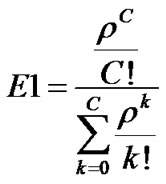
3.1. Erlang B Formula
Erlang B formula deals with probability of data loss un-
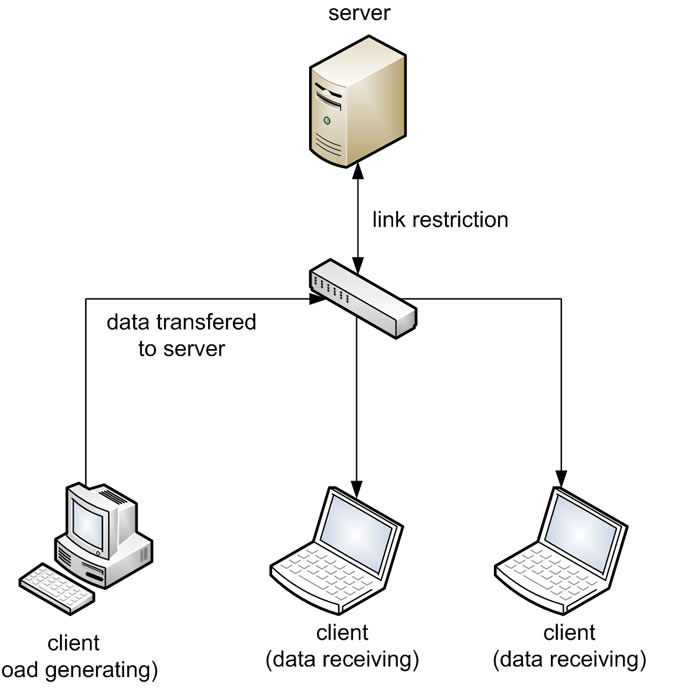
Figure 1. Tested model.
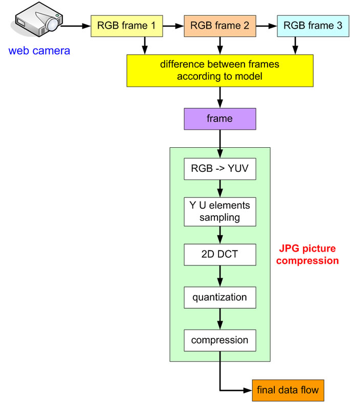
Figure 2. Video model with VBR data flow.
der link load [22]. Its basic form is (2):
 (2)
(2)
Symbol meanings are:
•  - total load [%]
• C - number of links.
We revised formula (2) into form (3), which is more appropriate for calculations. From this formula results relation of two parameters:
•  - link load in [%]
• C - link speed in Mbit/s.
 (3)
(3)
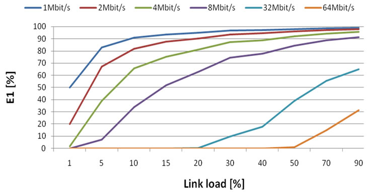
Figure 3. Data loss probability in the case of constant bandwidth.
From Figure 3. results:
• Probability of loss increases with link load.
• With increasing bandwidth data loss is decreasing.
After revision and modification of Erlang formula with parameter m, (number of sources in common path) we used formula (4) for further calculations. Other parameters stayed the same.
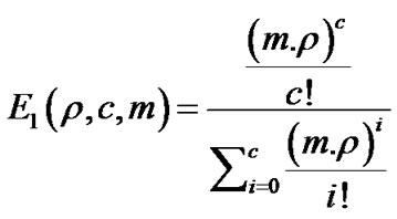 (4)
(4)
Common path means that more flows are transferred through one way. Link bandwidth requirements are then summarized together.
From Figure 4. results:
• Under low link load with increasing number of sources is data loss probability reduced.
• Under higher link load (5%) this difference is not as much notable and the loss is gradually flatten.
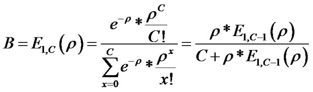
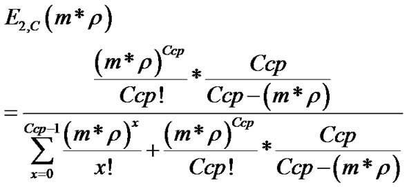
3.2. Erlang C Formula
Probability of waiting the requests in queue is described by second Erlang formula (5).
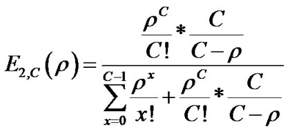 (5)
(5)
For calculations, a form without factorials is preferable. In case that , we can rewrite formula to (6).
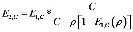 (6)
(6)
From Figure 5. results:
• With increasing link load, probability of insertion into waiting queue also increases.
• With increasing bandwidth, probability of insertion into waiting queue decreases.
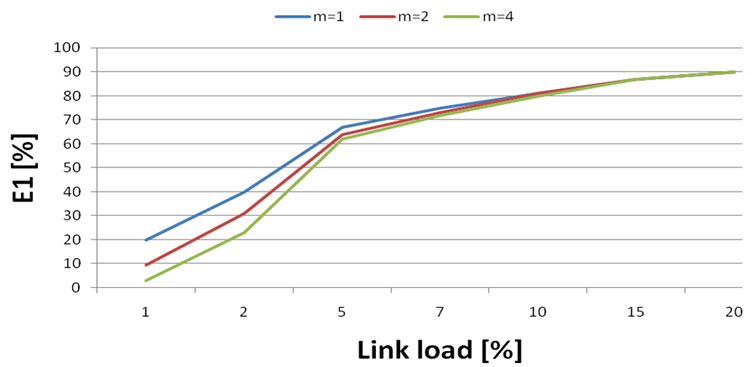
Figure 4. Data loss probability in the case of constant bandwidth 2 Mbit/s and m flows.
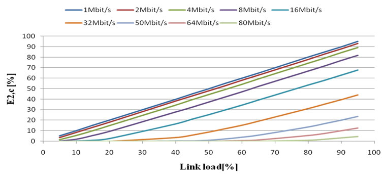
Figure 5. Probability of insertion into waiting queue in case of constant bandwidth.
• With low link speeds (under 16 Mbit/s), the behaviour of probabilities is nearly linear.
Formula (6) extended by m parameter:
 (7)
(7)
where:
•  - link load [%].
• Ccp – link speed (for common path) in Mbit/s.
• m – number of sources.
From Figure 6. results:
• With increasing link load and constant bandwidth, the probability of insertion into waiting queue increases.
• With higher common path utilization, the probability of insertion into waiting queue is also higher.
• With increasing of common path bandwidth, it is possible multiple use of traffic links also with higher load.
• Common path bandwidth affects slope of probability of insertion into waiting queue.
4. Results Comparison
When comparing results from MATLAB simulations and real measurements, it is necessary to consider VBR video characteristics and used queues for traffic shaping. For
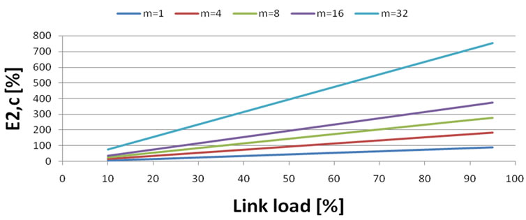
Figure 6. Probability of insertion into waiting queue in case of common usage of 4 Mbit/s link.
simulation of formula B we used RED mechanism, because packets were dropped after reaching maximum queue length. Formula C uses SFQ mechanism, which does not drop packets, but inserts them into waiting queue.
4.1. Erlang B Formula
Firstly we measured loss in relation to link load at 2 Mbit/s, 4 Mbit/s and 8 Mbit/s link capacity. In Figure 7. we can see that graphs look like in simulations (section 3.1), but values of loss are much lower (loss decreases with link capacity). This is caused by VBR video characteristics, where loss does not occurs until reaching link capacity.
Next testing of formula B was by common usage of the link (Figures 8, 9 and 10). Each flow was transferred with some time delay against other flows. This way we prevented overloading of the link by VBR video. From this measurement results:
• With constant network load and increasing bandwidth it is possible to raise the number of sources.
• With constant load and bandwidth, loss increases with number of sources per link.
• With increasing link capacity we can add number of sources per one path.
4.2. Erlang C Formula
The method was the same as with Erlang B formula, ex-
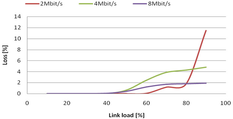
Figure 7. Loss probability in case of constant bandwidth.
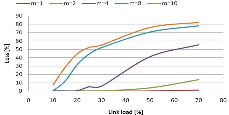
Figure 8. Loss probability in case of 2 Mbit/s bandwidth and m flows.
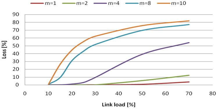
Figure 9. Loss probability in case of 4 Mbit/s bandwidth and m flows.
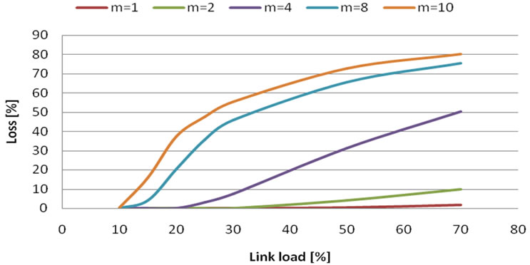
Figure 10. Loss probability in case of 8 Mbit/s bandwidth and m flows.
cept for the fact, that data which came later, were labeled as loss, because they went to waiting queue.
From Figure 11. results:
• SFQ waiting queue is a better choice for VBR video, because of its better handle with high-peak rate .
• Compared to MATLAB simulations, loss is under 5% even until full network usage. This is caused by SFQ queue and VBR data model.
We also tried common path usage with Erlang C formula (Figures12, 13 and 14). Flows were put together in the same way as with Erlang B formula. Simulation results:
• Graphs are now comparable with MATLAB simulations (the curves look similar), but with lower probability of loss.
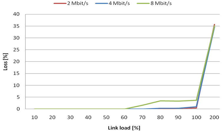
Figure 11. Loss probability in case of constant bandwidth.
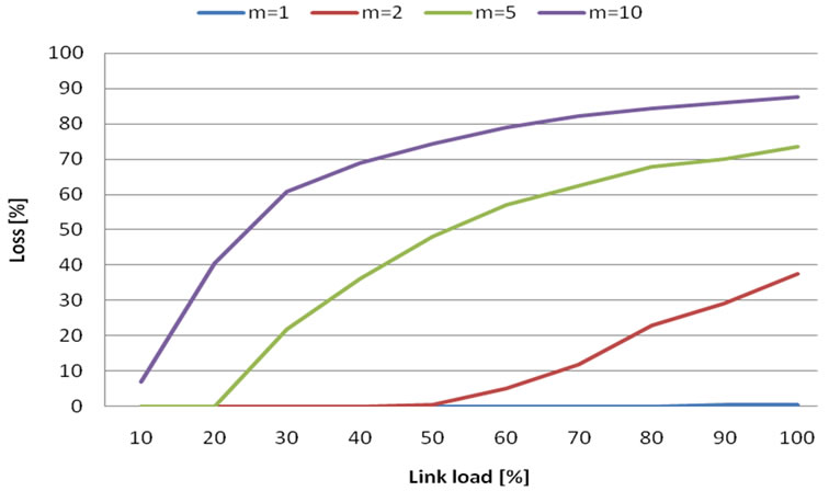
Figure 12. Loss probability in case of m flows and 2 Mbit bandwidth.
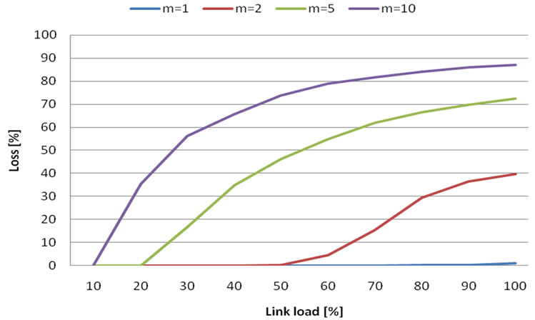
Figure 13. Loss probability in case of m flows and 4 Mbit bandwidth.
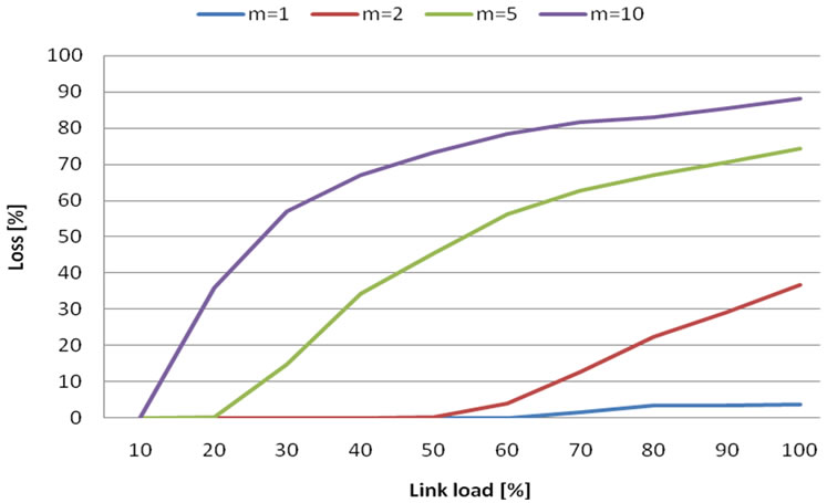
Figure 14. Loss probability in case of m flows and 8 Mbit bandwidth.
• Similar to Erlang B formula, it is useful to put together more flows into one path.
• With increasing bandwidth, we can put together more flows into one path and assure acceptable loss (based on SLA).
5. Conclusions
The purpose of this work was to evaluate utilization of Erlang B and C formulas in IP environment with VBR video data flow. We have showed the difference between two link shaping methods and we found out that SFQ is more appropriate for usage. Erlang formula is then a good choice for VBR data flow calculations with respect to loss dependencies. It is possible to estimate network behavior under load with these formulas. These formulas give us only approximately estimation. Loss probabilities were not exactly as predicted by calculations, but lower. It is caused by VBR video characteristics and data transfer method in IP networks. Calculations and real measurements have shown advantages of effective link load. Putting more VBR flows together into one link has greatly improved effectiveness of data transfer.
6. Acknowledgements
This work is a part of research activities conducted at Slovak University of Technology Bratislava, Faculty of Electrical Engineering and Information Technology, Department of Telecommunications, within the scope of the projects VEGA No. 1/0565/09, Modelling of traffic parameters in NGN telecommunication networks and services and ITMS 26240120029 “Support for Building of Centre of Excellence for SMART technologies, systems and services II”.
7. References
[1] L. Dostálek and A. Kabelová, “Understanding TCP/IP,” Packt, Birmingham, 2006.
[2] A. Kováč, M. Halás and M. Vozňák, “Impact of Jitter on Speech Guality Estimation in Modified E-Model,” 12th International Conference Research in Telecommunication Technology, Velké Losiny, 8-10 September 2010, p. 225.
[3] T. Mišuth and I. Baroňák, “Performance Forecast of Contact Centre with Differently Experienced Agents,” Elektrorevue, Vol. 15, No. 97, 2010.
[4] I. Baroňák and J. Mičuch, “Preventive Methods Supporting QOS in IP,” New Information and Multimedia Technologies. NIMT—2009, Brno University of Technology, Brno, 17-18 September 2009, pp. 15-23.
[5] T. Balogh, D. Luknárová and M. Medvecký, “Performance of Round Robin-Based Queue Scheduling Algorithms,” The Third International Conference on Communication Theory, Reliability and Quality of Service, Athens, 13-19 June 2010, pp. 156-161.
[6] C. Wootton, “A Practial Guide to Video and Audio Compression,” Focal Press, Oxford, 2005.
[7] Š. Peško, “System Queuing Theory,” 2001. http://frcatel.fri.uniza.sk/users/pesko/OA2/oa2m.pdf
[8] J. F. Hayes, et al., “Modeling and Analysis of Telecommunications Networks,” Wiley Interscience, New York, 2004.
[9] V. B. Iversen, “Teletraffic Engineering Handbook,” COM Centre, Technical University of Denmark, Copenhagen, 2001.
[10] T. Graf, G. Maxwell and R. Mook, “Linux Advanced Routing & Traffic Control,” 2004. http://lartc.org/.
[11] K. Thomas, “Beginning Ubuntu Linux from Novice to Professional,” Apress, New York City, 2006.
[12] M. Bauer, “Building Secure Servers with LINUX,” O’Reilly Media, Sebastopol, 2003.
[13] S. Hunger, “Debian GNU-Linux Bible,” Hungary Minds, New York, 2001.
[14] A. Kist, “Erlang B as a Performance Model for IP Flows Networks,” 15th IEEE International Conference on Networks, Adelaide, 19-21 November 2007, pp. 37-41.
[15] M. Hofmann and L. Beaumont, “Content Networking,” MK Publishers, St Petersburg, 2005, pp. 834-836.
[16] G. Davies, “Designing and Developing Scalable IP Network,” John Wiley & Sons Ltd, Hoboken, 2004.
[17] G. Held, “Ethernet Networks—Fourth Edition,” John Wiley & Sons Ltd, Hoboken, 2003.
[18] S. Plumley, “Home Networking Bible,” John Wiley & Sons Ltd, Hoboken, 2004.
[19] V. Pirogov, “Mastership in Assembler Language,” Computer Press, Brno, 2005.
[20] J. Pirkl, “Network programming in Windows and Internet Programming,” Kopp, České Budějovice, 2001.
[21] R. Chalupa, “1001 Tips and Tricks for Visual C++,” Computer Press, Brno, 2003, ISBN 1-904811-71-0.
[22] I. Baroňák, “Lecture on Switching Systems II,” 08/09, FEI STU Bratislava. http://www.ktl.elf.stuba.sk/~baronak/PEDAGOGIKA.htm