Journal of Water Resource and Protection
Vol. 3 No. 1 (2011) , Article ID: 3778 , 10 pages DOI:10.4236/jwarp.2011.31006
Time Series Modeling of River Flow Using Wavelet Neural Networks
Deltaic Regional Center, National Institute of Hydrology Kakinada, Andhra Pradesh, India
E-mail: krishna_nih@rediffmail.com
Received September 24, 2009; revised October 18, 2010; accepted November 19, 2010
Keywords: Time Series, River Flow, Wavelets, Neural Networks
ABSTRACT
A new hybrid model which combines wavelets and Artificial Neural Network (ANN) called wavelet neural network (WNN) model was proposed in the current study and applied for time series modeling of river flow. The time series of daily river flow of the Malaprabha River basin (Karnataka state, India) were analyzed by the WNN model. The observed time series are decomposed into sub-series using discrete wavelet transform and then appropriate sub-series is used as inputs to the neural network for forecasting hydrological variables. The hybrid model (WNN) was compared with the standard ANN and AR models. The WNN model was able to provide a good fit with the observed data, especially the peak values during the testing period. The benchmark results from WNN model applications showed that the hybrid model produced better results in estimating the hydrograph properties than the latter models (ANN and AR).
1. Introduction
Water resources planning and management requires, output from hydrological studies. These are mainly in the form of estimation or forecasting of the magnitude of hydrological variables like precipitation, stream flow and groundwater levels using historical data. Forecasting of hydrological variables especially stream flow is utmost important to provide a warning of the extreme flood or drought conditions and helps to develop operation systems of multipurpose reservoirs. Similarly, groundwater level modeling is useful for consumptive use studies for better watershed management.
Time series modeling for either data generation or forecasting of hydrological variables is an important step in the planning and management of water resources. Most of the time series modeling procedures fall within the framework of multivariate Auto Regressive Moving Average (ARMA) model [1]. Traditionally, ARMA models have been widely used for modeling water resources time-series modeling [2]. The time series models are used to describe the stochastic structure of the time sequence of a hydrological variable measured over time. Time-series models are more practical than conceptual models because it is not essential to understand the internal structure of the physical processes that are taking place in the system being modeled. Time series analysis requires mapping complex relationships between input(s) and output(s), since the forecasted values are mapped as a function of observed patterns in the past. On the other hand, classical non-linear techniques typically require large amounts of exogenous data, which are not always available [3]; some non-linear approaches outperform the linear techniques, as periodic gamma autoregressive processes (PGAR) for instance [4], but they can only be applied to a single site, i.e., they are limited to be univariate models. Owing to the difficulties associated with non-linear model structure identification and parameter estimation, very few truly non-linear system theoretic hydrologic models have been reported [5-7]. It seems necessary that nonlinear models such as neural networks, which are suited to complex nonlinear problems, be used for the time series modeling of river flow.
Artificial Neural Networks (ANN) has been used successfully to overcome many difficulties in time series modeling of river flow. Time series modeling using ANN has been a particular focus of interest and better performing models have been reported in a diverse set of fields that include rainfall-runoff modeling [8-12] and groundwater level prediction [13-16]. It is also reported that ANN models are not very satisfied in precision for forecasting because it considered only few aspects of time series property [17]. In order to raise the forecasted precision and lengthen the forecasted time, an alternative model should be envisaged. In this paper, a new hybrid model called wavelet neural network model (WNN), which is the combination of wavelet analysis and ANN, has been proposed. The advantage of the wavelet technique is that it provides a mathematical process for decomposing a signal into multi-levels of details and analysis of these details can be done. Wavelet analysis can effectively diagnose signals of main frequency component and abstract local information of the time series. In the past decade, wavelet theory has been introduced to signal processing analysis. In recent years, the wavelet transforms has been successfully applied to wave data analysis and other ocean engineering applications [18,19].
In recent years, wavelet theory has been introduced in the field of hydrology [17,20-22]. Wavelet analysis has recently been identified as a useful tool for describing both rainfall and runoff time-series [21,23-26]. By coupling the wavelet method with the traditional AR model, the Wavelet-Autoregressive model (WARM) is developed for annual rainfall prediction [27]. Coulibaly [28] used the wavelet analysis to identify and describe variability in annual Canadian stream flows and to gain insights into the dynamical link between the stream flows and the dominant modes of climate variability in the Northern Hemisphere. Due to the similarity between wavelet decomposition and one hidden layer neural network, the idea of combining both wavelet and neural network has resulted recently in formulation of wavelet neural network, which has been used in various fields [29]. Results show that, the training and adaptation efficiency of the wavelet neural network is better than other networks. Dongjie [30] used a combination of neural networks and wavelet methods to predict ground water levels. Aussem [31] used a Dynamical Recurrent Neural Network (DRNN) on each resolution scale of the sunspot time series resulting from the wavelet decomposed series with the Temporal Recurrent Back propagation (TRBP) algorithm. Partal [32] used a conjunction model (wavelet-neurofuzzy) to forecast the Turkey daily precipitation. The observed daily precipitations are decomposed to some sub series by using Discrete Wavelet Transform (DWT) and then appropriate sub series are used as inputs to neurofuzzy models for forecasting of daily precipitations.
In this paper, an attempt has been made to forecast the time series of Daily River flow by developing wavelet neural network (WNN) models. Time series of river flow was decomposed into wavelet sub-series by discrete wavelet transform. Then, neural network model is constructed with wavelet sub-series as input, and the original time series as output. Finally, the forecasting performance of WNN model was compared with the ANN and AR models.
2. Methods of Analysis
2.1. Wavelet Analysis
The wavelet analysis is an advance tool in signal processing that has attracted much attention since its theoretical development [33]. Its use has increased rapidly in communications, image processing and optical engineering applications as an alternative to the Fourier transform in preserving local, non-periodic and multiscaled phenomena. The difference between wavelets and Fourier transforms is that wavelets can provide the exact locality of any changes in the dynamical patterns of the sequence, whereas the Fourier transforms concentrate mainly on their frequency. Moreover, Fourier transform assume infinite-length signals, whereas wavelet transforms can be applied to any kind and size of time series, even when these sequences are not homogeneously sampled in time [34]. In general, wavelet transforms can be used to explore, denoise and smoothen time series, aid in forecasting and other empirical analysis.
Wavelet analysis is the breaking up of a signal into shifted and scaled versions of the original (or mother) wavelet. In wavelet analysis, the use of a fully scalable modulated window solves the signal-cutting problem. The window is shifted along the signal and for every position the spectrum is calculated. Then this process is repeated many times with a slightly shorter (or longer) window for every new cycle. In the end, the result will be a collection of time-frequency representations of the signal, all with different resolutions. Because of this collection of representations we can speak of a multiresolution analysis. By decomposing a time series into timefrequency space, one is able to determine both the dominant modes of variability and how those modes vary in time. Wavelets have proven to be a powerful tool for the analysis and synthesis of data from long memory processes. Wavelets are strongly connected to such processes in that the same shapes repeat at different orders of magnitude. The ability of the wavelets to simultaneously localize a process in time and scale domain results in representing many dense matrices in a sparse form.
2.2. Discrete Wavelet Transform (DWT)
The basic aim of wavelet analysis is both to determine the frequency (or scale) content of a signal and to assess and determine the temporal variation of this frequency content. This property is in complete contrast to the Fourier analysis, which allows for the determination of the frequency content of a signal but fails to determine frequency timedependence. Therefore, the wavelet transform is the tool of choice when signals are characterized by localized high frequency events or when signals are characterized by a large numbers of scale-variable processes. Because of its localization properties in both time and scale, the wavelet transform allows for tracking the time evolution of processes at different scales in the signal.
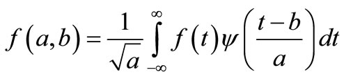
The wavelet transform of a time series f(t) is defined as
 (1)
(1)
where  is the basic wavelet with effective length (t) that is usually much shorter than the target time series f(t). The variables are a and b, where a is the scale or dilation factor that determines the characteristic frequency so that its variation gives rise to a ‘spectrum’; and b is the translation in time so that its variation represents the ‘sliding’ of the wavelet over f(t). The wavelet spectrum is thus customarily displayed in time-frequency domain. For low scales i.e. when
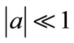 , the wavelet function is highly concentrated (shrunken compressed) with frequency contents mostly in the higher frequency bands. Inversely, when
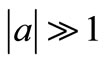 , the wavelet is stretched and contains mostly low frequencies. For small scales, we obtain thus a more detailed view of the signal (also known as a “higher resolution”) whereas for larger scales we obtain a more general view of the signal structure.
The original signal X(n) passes through two complementary filters (low pass and high pass filters) and emerges as two signals as Approximations (A) and Details (D). The approximations are the high-scale, low frequency components of the signal. The details are the low-scale, high frequency components. Normally, the low frequency content of the signal (approximation, A) is the most important part. It demonstrates the signal identity. The high-frequency component (detail, D) is nuance. The decomposition process can be iterated, with successive approximations being decomposed in turn, so that one signal is broken down into many lower resolution components (Figure 1).
2.3. Mother Wavelet
The choice of the mother wavelet depends on the data to be analyzed. The Daubechies and Morlet wavelet transforms are the commonly used “Mother” wavelets. Daubechies wavelets exhibit good trade-off between parsimony and information richness, it produces the identical events across the observed time series and appears in so many different fashions that most prediction models are unable to recognize them well [35]. Morlet wavelets, on the other hand, have a more consistent response to similar events but have the weakness of generating many more inputs than the Daubechies wavelets for the prediction models.
An ANN, can be defined as a system or mathematical model consisting of many nonlinear artificial neurons running in parallel, which can be generated, as one or multiple layered. Although the concept of artificial neurons was first introduced by McCulloch and Pitts [36], the major applications of ANN’s have arisen only since the development of the back-propagation method of training by Rumelhart [37]. Following this development, ANN research has resulted in the successful solution of some complicated problems not easily solved by traditional modeling methods when the quality/quantity of data is very limited. ANN models are ‘black box’ models with particular properties, which are greatly suited to dynamic nonlinear system modeling. The main advantage of this approach over traditional methods is that it does not require the complex nature of the underlying process under consideration to be explicitly described in mathematical form. ANN applications in hydrology vary, from real-time to event based modeling.
The most popular ANN architecture in hydrologic modeling is the multilayer perceptron (MLP) trained with BP algorithm [8,9]. A multilayer perceptron network consists of an input layer, one or more hidden layers of computation nodes, and an output layer. The number of input and output nodes is determined by the
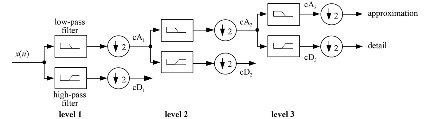
Figure 1. Diagram of multiresolution analysis of signal.
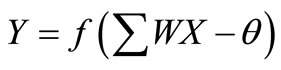
nature of the actual input and output variables. The number of hidden nodes, however, depends on the complexity of the mathematical nature of the problem, and is determined by the modeler, often by trial and error. The input signal propagates through the network in a forward direction, layer by layer. Each hidden and output node processes its input by multiplying each of its input values by a weight, summing the product and then passing the sum through a nonlinear transfer function to produce a result. For the training process, where weights are selected, the neural network uses the gradient descent method to modify the randomly selected weights of the nodes in response to the errors between the actual output values and the target values. This process is referred to as training or learning. It stops when the errors are minimized or another stopping criterion is met. The BPNN can be expressed as
 (2)
(2)
where X = input or hidden node value; Y = output value of the hidden or output node; f (.) = transfer function; W = weights connecting the input to hidden, or hidden to output nodes; and θ = bias (or threshold) for each node.
3. Method of Network Training
Levenberg-Marquardt method (LM) was used for the training of the given network. Levenberg-Marquardt method (LM) is a modification of the classic Newton algorithm for finding an optimum solution to a minimization problem. In practice, LM is faster and finds better optima for a variety of problems than most other methods [38]. The method also takes advantage of the internal recurrence to dynamically incorporate past experience in the training process [39].
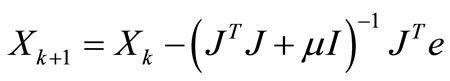
The Levenberg-Marquardt algorithm is given by
 (3)
(3)
where, X is the weights of neural network, J is the Jacobian matrix of the performance criteria to be minimized, m is a learning rate that controls the learning process and e is residual error vector.
If scalar m is very large, the above expression approximates gradient descent with a small step size; while if it is very small; the above expression becomes GaussNewton method using the approximate Hessian matrix. The Gauss-Newton method is faster and more accurate near an error minimum. Hence we decrease m after each successful step and increase only when a step increases the error. Levenberg-Marquardt has great computational and memory requirements, and thus it can only be used in small networks. It is faster and less easily trapped in local minima than other optimization algorithms.
3.1. Selection of Network Architecture
Increasing the number of training patterns provide more information about the shape of the solution surface, and thus increases the potential level of accuracy that can be achieved by the network. A large training pattern set, however can sometimes overwhelm certain training algorithms, thereby increasing the likelihood of an algorithm becoming stuck in a local error minimum. Consequently, there is no guarantee that adding more training patterns leads to improve solution. Moreover, there is a limit to the amount of information that can be modeled by a network that comprises a fixed number of hidden neurons. The time required to train a network increases with the number of patterns in the training set. The critical aspect is the choice of the number of nodes in the hidden layer and hence the number of connection weights.
Based on the physical knowledge of the problem and statistical analysis, different combinations of antecedent values of the time series were considered as input nodes. The output node is the time series data to be predicted in one step ahead. Time series data was standardized for zero mean and unit variation, and then normalized into 0 to 1. The activation function used for the hidden and output layer was logarithmic sigmoidal and pure linear function respectively. For deciding the optimal hidden neurons, a trial and error procedure started with two hidden neurons initially, and the number of hidden neurons was increased up to 10 with a step size of 1 in each trial. For each set of hidden neurons, the network was trained in batch mode to minimize the mean square error at the output layer. In order to check any over-fitting during training, a cross validation was performed by keeping track of the efficiency of the fitted model. The training was stopped when there was no significant improvement in the efficiency, and the model was then tested for its generalization properties. Figure 2 shows the multilayer perceptron (MLP) neural network architecture when the original signal taken as input of the neural network architecture.
3.2. Method of Combining Wavelet Analysis with ANN
The decomposed details (D) and approximation (A) were taken as inputs to neural network structure as shown in Figure 3. In Figure 3, i is the level of decomposition varying from 1 to I and j is the number of antecedent values varying from 0 to J and N is the length of the time series. To obtain the optimal weights (parameters) of the neural network structure, LM back-propagation algorithm has been used to train the network. A standard MLP with a logarithmic sigmoidal transfer function for the hidden
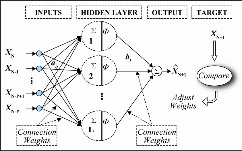
Figure 2. Signal data based multilayer perceptron (MLP) neural network structure.
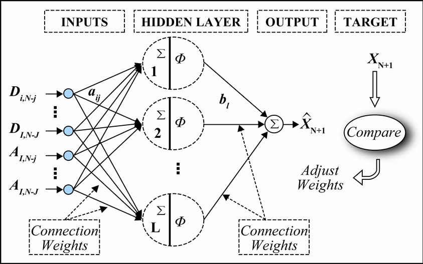
Figure 3. Wavelet based multilayer perceptron (MLP) neural network structure.
layer and linear transfer function for the output layer were used in the analysis. The number of hidden nodes was determined by trial and error procedure. The output node will be the original value at one step ahead.
3.3. Linear Auto-Regressive (AR) Modeling
A common approach for modeling univariate time series is the autoregressive (AR) model:
 (4)
(4)
where Xt is the time series, At is white noise, and
 (5)
(5)
where  is the mean of the time series. An autoregressive model is simply a linear regression of the current value of the series against one or more prior values. AR models can be analyzed with linear least squares technique. They also have a straightforward interpretation. The determination of the model order can be estimated by examining the plots of Auto Correlation Function (ACF) and Partial Auto Correlation Function (PACF). The number of non-zero terms (i.e. outside confidence bands) in PACF suggests the order of the AR model. An AR (k) model will be implied by a sample PACF with k non-zero terms, and the terms in the sample ACF will decay slowly towards zero. From ACF and PACF analysis for river flow, the order of the AR model is selected as 1.
1) Performance Criteria The performance of various models during calibration and validation were evaluated by using the statistical indices: the Root Mean Squared Error (RMSE), Correlation Coefficient (R), Coefficient of Efficiency (COE) and Persistence Index (PI).
2) Study Area In this paper, a hybrid model wavelet neural network (WNN) used to forecast the river flow of the Malaprabha River basin (Figure 4) in Karnataka state of India. The river Malaprabha is one of the tributary of river Krishna, originated from Kanakumbi in the Western Ghats at an altitude of 792.48 m in Belgaum district of Karnataka State. The river flows in an easterly direction and joins the River Krishna. The Malaprabha river upto Khanapur gauging station was considered for the present study. It is having a total catchment area of 520 Sq.km. and lies between 150 30' to 150 50' N latitude and 740 12' to 740 32' E longitude. About 60% of the basin was covered with forests covering upstream area of the basin and northern part of the basin is used for agricultural purpose. Major portion of the catchment is covered with tertiary basaltic rock, whereas, the sedimentary rocks have confined to the southeastern part of the catchment. Most of the rainfall of the basin experiences from southwest monsoon. The average annual precipitation is 2337 mm from seven rain gauges, which are uniformly distributed throughout the basin (Figure 4). The average daily river flow data of 11 years (1986-1996) used for the current study. The maximum value of the testing data set is fall within the training data set limit. This means that the trained neural network models do not face difficulties in making extrapolation.
4. Development of Wavelet Neural Network Model
The original time series was decomposed into Details and Approximations a certain number of sub-time series
 by wavelet transform algorithm.
These play different role in the original time series and the behavior of each sub-time series is distinct [17]. So the contribution to original time series varies from each
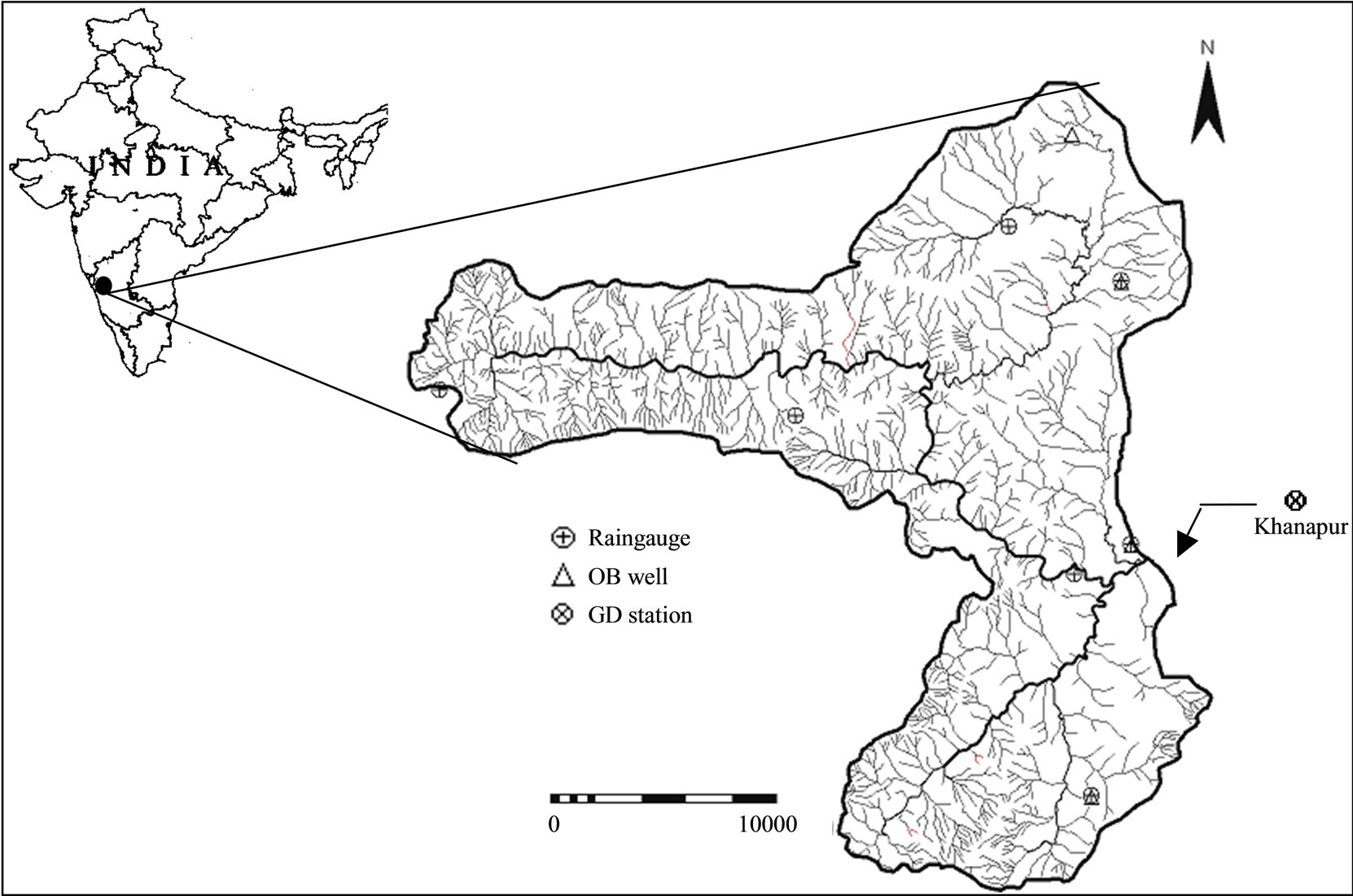
Figure 4. Location of study area.
other. The decomposition process can be iterated, with successive approximations being decomposed in turn, so that one signal is broken down into many lower resolution components, tested using different scales from 1 to 10 with different sliding window amplitudes. In this context, dealing with a very irregular signal shape, an irregular wavelet, the Daubechies wavelet of order 5 (DB5), has been used at level 3. Consequently, D1, D2, D3 were detail time series, and A3 was the approximation time series.
An ANN was constructed in which the sub-series {D1, D2, D3, A3} at time t are input of ANN and the original time series at t + T time are output of ANN, where T is the length of time to forecast. The input nodes are the antecedent values of the time series and were presented in Table 1. The Wavelet Neural Network model (WNN) was formed in which the weights are learned with Feed forward neural network with Back Propagation algorithm. The number of hidden neurons for BPNN was determined by trial and error procedure.
5. Results and Discussion
To forecast the river flow at Khanapur gauging station of Malaprabha River (Figure 4), the daily stream flow data of 11 years was used. The first seven years (1986-92) data were used for calibration of the model, and the remaining four years (1993-96) data were used for validation. The model inputs (Table 1) were decomposed by wavelets and decomposed sub-series were taken as input to ANN and the original river flow value in one day ahead as output. ANN was trained using backpropagation with LM algorithm. The optimal number of hidden neurons was determined as three by trial and error procedure.
The performance of various models estimated to forecast the river flow was presented in Table 2. From Table 2, it was found that low RMSE values (8.24 to 18.60 m3/s) for WNN models when compared to ANN and AR (1) models. It was observed that WNN models estimated the peak values of river flow to a reasonable accuracy (peak flow during the study was 774 m3/s). From Table 2, it was observed that the WNN model having four antecedent values of the time series, estimated minimum
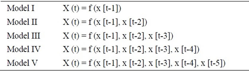
Table 1. Model inputs.
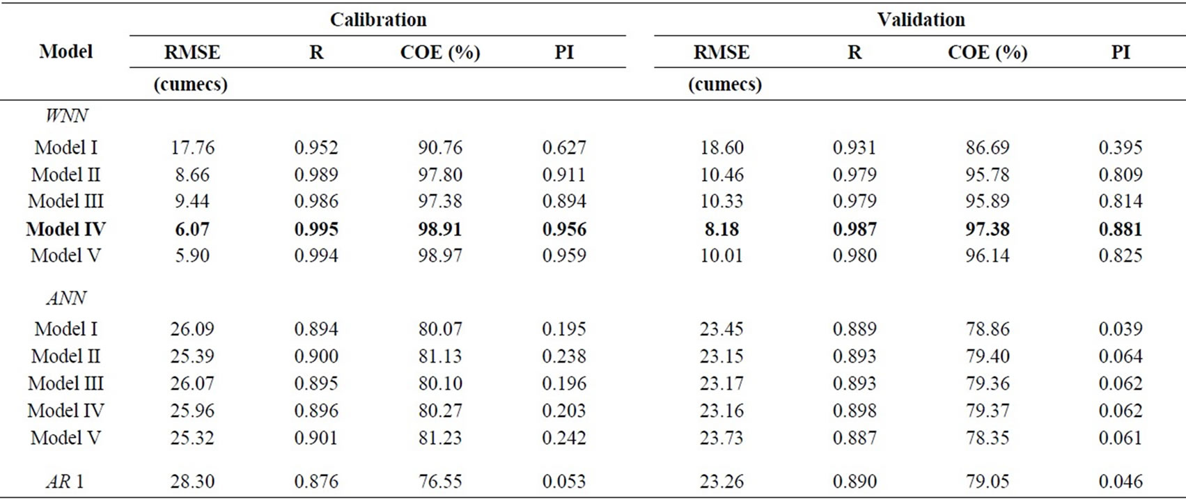
Table 2. Goodness of fit statistics of the forecasted river flow for the calibration and validation period.
RMSE (8.24 m3/s), high correlation coefficient (0.9870), highest efficiency (> 97%) and a high PI value of 0.881 during the validation period. The model IV of WNN was selected as the best-fit model to forecast the river flow in one-day advance.
An analysis to assess the potential of each of the model to preserve the statistical properties of the observed flow series was carried out and reveals that the flow series computed by the WNN model reproduces the first three statistical moments (i.e. mean, standard deviation and skewness) better than that computed by the ANN model. The values of the first three moments for the observed and modeled flow series for the validation period were presented in Table 3 for comparison. In Table 3, AR model performance was not presented because of its low efficiency compared to other models. Table 3 depicts the percentage error in annual peak flow estimates for the validation period for both models. From Table 3 it is found that the WNN model improves the annual peak flow estimates and the error was limited to 18%. However, ANN models tend to underestimate the peak flow up to 55% error in peak estimation.
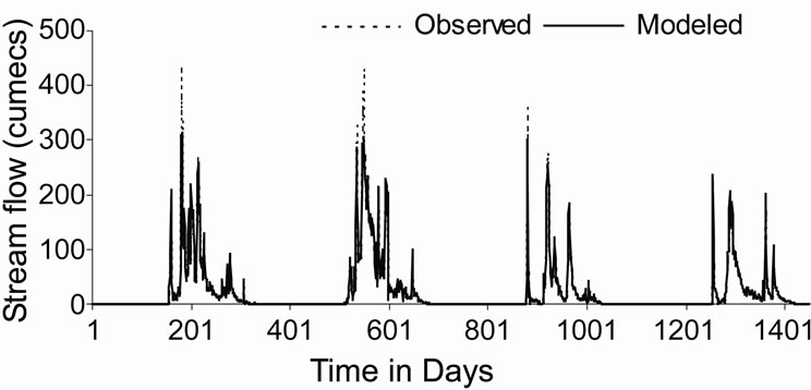
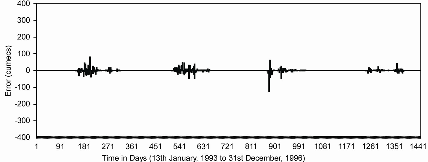
Figure 5 shows the observed and modeled hydrographs for WNN and ANN models. It was found that values modeled from WNN model correctly matched with the observed values, whereas, ANN model underestimated the observed values. The distribution of error along the magnitude of river flow computed by WNN and ANN models during the validation period has been presented in Figure 6. From Figure 6, it was observed that the estimation of peak flow was very good as the error is minimum when compared with ANN model. Figure 7 shows the scatter plot between the observed and modeled flows by WNN and ANN. It was observed that the flow forecasted by WNN models were very much close to the 45 degrees line. From this analysis, it was worth to mention that the performance of WNN was much better than ANN and AR models in forecasting the river flow in one-day advance.
6. Conclusions
This paper reports a hybrid model called wavelet based neural network model for time series modeling of river flow. The proposed model is a combination of wavelet analysis and artificial neural network (WNN). Wavelet decomposes the time series into multi-levels of details and it can adopt multi-resolution analysis and effectively
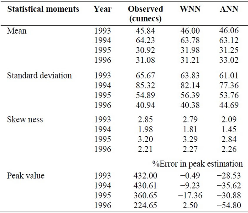
Table 3. Statistical moments of the observed and modeled river flow series during validation period.
 (a)
(a)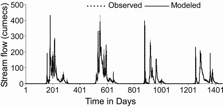 (b)
(b)
Figure 5. Plot of observed and modeled hydrographs for (a) WNN and (b) ANN model for the validation period.
 (a)
(a)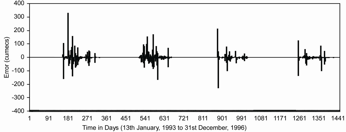 (b)
(b)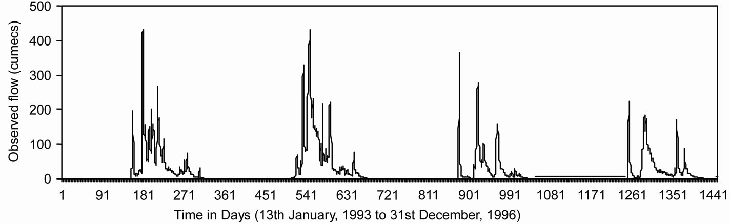 (c)
(c)
Figure 6. Distribution of error plots along the magnitude of river flow for (a) WNN model and (b) ANN model during validation period.
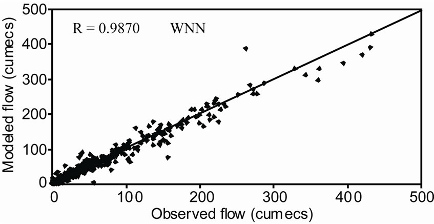
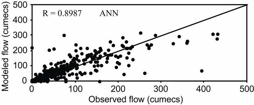
Figure 7. Scatter plot between observed and modeled river flow during validation period.
diagnose the main frequency component of the signal and abstract local information of the time series. The proposed WNN model was applied to daily river flow of Malaprabha river basin in Belgaum district of Karnataka State, India. The time series data of river flow was decomposed into sub series by DWT. Each of sub-series plays distinct role in original time series. Appropriate sub-series of the variable used as inputs to the ANN model and original time series of the variable as output. From the current study it is found that the proposed wavelet neural network model is better in forecasting river flow in Malaprabha basin. In the analysis, original signals are represented in different resolution by discrete wavelet transformation, therefore, the WNN forecasts are more accurate than that obtained directly by original signals.
REFERENCES
- H. Raman and N. Sunil Kumar, “Multivariate Modeling of Water Resources Time Series Using Artificial Neural Networks,” Journal of Hydrological Sciences, Vol. 40, No. 4, 1995, pp. 145-163. doi:10.1080/02626669509491401
- H. R. Maier and G. C. Dandy, “Determining Inputs for Neural Network Models of Multivariate Time Series,” Microcomputers in Civil Engineering, Vol. 12, 1997, pp. 353-368.
- M. C. Deo and K. Thirumalaiah, “Real Time Forecasting Using Neural Networks: Artificial Neural Networks in Hydrology,” In: R. S. Govindaraju and A. Ramachandra Rao, Kluwer Academic Publishers, Dordrecht, 2000, pp. 53-71.
- B. Fernandez and J. D. Salas, “Periodic Gamma Autoregressive Processes for Operational Hydrology,” Water Resources Research, Vol. 22, No. 10, 1986, pp. 1385- 1396. doi:10.1029/WR022i010p01385
- S. L. S. Jacoby, “A Mathematical Model for Non-Linear Hydrologic Systems,” Journal of Geophysics Research, Vol. 71, No. 20, 1966, pp. 4811-4824.
- J. Amorocho and A. Brandstetter, “A Critique of Current Methods of Hydrologic Systems Investigations,” Eos Transactions of AGU, Vol. 45, 1971, pp. 307-321.
- S. Ikeda, M. Ochiai and Y. Sawaragi, “Sequential GMDH Algorithm and Its Applications to River Flow Prediction,” IEEE Transactions of System Management and Cybernetics, Vol. 6, No. 7, 1976, pp. 473-479. doi:10.1109/TSMC.1976.4309532
- ASCE Task Committee, “Artificial Neural Networks in hydrology-I: Preliminary Concepts,” Journal of Hydrologic Engineering, Vol. 5, No. 2, 2000(a), pp. 115-123.
- ASCE Task Committee, “Artificial Neural Networks in Hydrology-II: Hydrologic Applications,” Journal of Hydrologic Engineering, Vol. 5, No. 2, 2000(b), pp. 124- 137.
- D. W. Dawson and R. Wilby, “Hydrological Modeling Using Artificial Neural Networks,” Progress in Physical Geograpgy, Vol. 25, No. 1, 2001, pp. 80-108.
- S. Birikundavy, R. Labib, H. T. Trung and J. Rousselle, “Performance of Neural Networks in Daily Stream Flow Forecasting,” Journal of Hydrologic Engineering, Vol. 7, No. 5, 2002, pp. 392-398. doi:10.1061/(ASCE)1084-0699(2002)7:5(392)
- P. Hettiarachchi, M. J. Hall and A. W. Minns, “The Extrapolation of Artificial Neural Networks for the Modeling of Rainfall-Runoff Relationships,” Journal of Hydroinformatics, Vol. 7, No. 4, 2005, pp. 291-296.
- E. J. Coppola, M. Poulton, E. Charles, J. Dustman and F. Szidarovszky, “Application of Artificial Neural Networks to Complex Groundwater Problems,” Journal of Natural Resources Research, Vol. 12, No. 4, 2003(a), pp. 303- 320.
- E. J. Coppola, F. Szidarovszky, M. Poulton and E. Charles, “Artificial Neural Network Approach for Predicting Transient Water Levels in a Multilayered Groundwater System under Variable State, Pumping and Climate Conditions,” Journal of Hydrologic Engineering, Vol. 8, No. 6, 2003(b), pp. 348-359.
- P. C. Nayak, Y. R. Satyaji Rao and K. P. Sudheer, “Groundwater Level Forecasting in a Shallow Aquifer Using Artificial Neural Network Approach,” Water Resources Management, Vol. 20, No. 1, 2006, pp. 77-90. doi:10.1007/s11269-006-4007-z
- B. Krishna, Y. R. Satyaji Rao and T. Vijaya, “Modeling Groundwater Levels in an Urban Coastal Aquifer Using Artificial Neural Networks,” Hydrological Processes, Vol. 22, No. 12, 2008, pp. 1180-1188. doi:10.1002/hyp.6686
- D. Wang and J. Ding, “Wavelet Network Model and Its Application to the Prediction of Hydrology,” Nature and Science, Vol. 1, No. 1, 2003, pp. 67-71.
- S. R. Massel, “Wavelet Analysis for Processing of Ocean Surface Wave Records,” Ocean Engineering, Vol. 28, 2001, pp. 957-987. doi:10.1016/S0029-8018(00)00044-5
- M. C. Huang, “Wave Parameters and Functions in Wavelet Analysis,” Ocean Engineering, Vol. 31, No. 1, 2004, pp. 111-125. doi:10.1016/S0029-8018(03)00047-7
- L. C. Smith, D. Turcotte and B. L. Isacks, “Stream Flow Characterization and Feature Detection Using a Discrete Wavelet Transform,” Hydrological Processes, Vol. 12, No. 2, 1998, pp. 233-249. doi:10.1002/(SICI)1099-1085(199802)12:2<233::AID-HYP573>3.0.CO;2-3
- D. Labat, R. Ababou and A. Mangin, “Rainfall-Runoff Relations for Karstic Springs: Part II. Continuous Wavelet and Discrete Orthogonal Multiresolution Analyses,” Journal of Hydrology, Vol. 238, No. 3-4, 2000, pp. 149- 178. doi:10.1016/S0022-1694(00)00322-X
- P. Saco and P. Kumar, “Coherent Modes in Multiscale Variability of Stream Flow over the United States,” Water Resources Research, Vol. 36, No. 4, 2000, pp. 1049- 1067.doi:10.1029/1999WR900345
- P. Kumar and E. Foufoula-Georgiou, “A Multicomponent Decomposition of Spatial Rainfall Fields: Segregation of Largeand Small-Scale Features Using Wavelet Transforms,” Water Resources Research, Vol. 29, No. 8, 1993, pp. 2515-2532. doi:10.1029/93WR00548
- P. Kumar, “Role of Coherent Structure in the Stochastic Dynamic Variability of Precipitation,” Journal of Geophysical Research, Vol. 101, 1996, pp. 393-404. doi:10.1029/96JD01839
- K. Fraedrich, J. Jiang, F.-W. Gerstengarbe and P. C. Werner, “Multiscale Detection of Abrupt Climate Changes: Application to the River Nile Flood,” International Journal of Climatology, Vol. 17, No. 12, 1997, pp. 1301- 1315.doi:10.1002/(SICI)1097-0088(199710)17:12<1301::AID-JOC196>3.0.CO;2-W
- R. H. Compagnucci, S. A. Blanco, M. A. Filiola and P. M. Jacovkis, “Variability in Subtropical Andean Argentinian Atuel River: A Wavelet Approach,” Environmetrics, Vol. 11, No. 3, 2000, pp. 251-269. doi:10.1002/(SICI)1099-095X(200005/06)11:3<251::AID-ENV405>3.0.CO;2-0
- S. Tantanee, S. Patamatammakul, T. Oki, V. Sriboonlue and T. Prempree, “Coupled Wavelet-Autoregressive Model for Annual Rainfall Prediction,” Journal of Environmental Hydrology, Vol. 13, No. 18, 2005, pp. 1-8.
- P. Coulibaly, “Wavelet Analysis of Variability in Annual Canadian Stream Flows,” Water Resources Research, Vol. 40, 2004.
- F. Xiao, X. Gao, C. Cao and J. Zhang, “Short-Term Prediction on Parameter-Varying Systems by Multiwavelets Neural Network,” Lecture Notes in Computer Science, Springer-Verlag, Vol. 3630, No. 3611, 2005, pp. 139- 146.
- D. J. Wu, J. Wang and Y. Teng, “Prediction of Underground Water Levels Using Wavelet Decompositions and Transforms,” Journal of Hydro-Engineering, Vol. 5, 2004, pp. 34-39.
- A. Aussem and F. Murtagh, “Combining Neural Network Forecasts on Wavelet Transformed Series,” Connection Science, Vol. 9, No. 1, 1997, pp. 113-121. doi:10.1080/095400997116766
- T. Partal and O. Kisi, “Wavelet and Neuro-Fuzzy Conjunction Model for Precipitation Forecasting,” Journal of Hydrology, Vol. 342, No. 1-2, 2007, pp. 199-212. doi:10.1016/j.jhydrol.2007.05.026
- A. Grossmann and J. Morlet, “Decomposition of Hardy Functions into Square Integrable Wavelets of Constant shape,” SIAM Journal on Mathematical Analysis, Vol. 15, No. 4, 1984, pp. 723-736. doi:10.1137/0515056
- A. Antonios and E. V. Constantine, “Wavelet Exploratory Analysis of the FTSE ALL SHARE Index,” Preprint submitted to Economics Letters University of Durham, Durham, 2003.
- D. Benaouda, F. Murtagh, J. L. Starck and O. Renaud, “Wavelet-Based Nonlinear Multiscale Decomposition Model for Electricity Load Forecasting,” Neurocomputing, Vol. 70, No. 1-3, 2006, pp. 139-154. doi:10.1016/j.neucom.2006.04.005
- W. McCulloch and W. Pitts, “A Logical Calculus of the Ideas Immanent in Nervous Activity,” Bulletin of Mathematical Biophysics, Vol. 5, 1943, pp. 115-133. doi:10.1007/BF02478259
- D. E. Rumelhart, G. E. Hinton and R. J. Williams, “Learning Representations by Back-Propagating Errors,” Nature, Vol. 323, No. 9, 1986, pp. 533-536. doi:10.1038/323533a0
- M. T. Hagan and M. B. Menhaj, “Training Feed forward Networks with Marquardt Algorithm,” IEEE Transactions on Neural Networks, Vol. 5, No. 6, 1994, pp. 989- 993. doi:10.1109/72.329697
- P. Coulibaly, F. Anctil, P. Rasmussen and B. Bobee, “A Recurrent Neural Networks Approach Using Indices of Low-Frequency Climatic Variability to Forecast Regional Annual Runoff,” Hydrological Processes, Vol. 14, No. 15, 2000, pp. 2755-2777. doi:10.1002/1099-1085(20001030)14:15<2755::AID-HYP90>3.0.CO;2-9