Advances in Pure Mathematics
Vol.4 No.7(2014), Article ID:48248,16 pages
DOI:10.4236/apm.2014.47045
Best Response Analysis in Two Person Quantum Games
Department of Mathematics, Texas A & M University—Kingsville, Kingsville, Texas, USA
Email: azharms2012@gmail.com, aden.ahmed@tamuk.edu
Received 25 May 2014; revised 25 June 2014; accepted 2 July 2014
ABSTRACT
In this paper, we find particular use for a maximally entangled initial state that produces a quan-tized version of two player two strategy games. When applied to a variant of the well-known game of Chicken, our construction shows the existence of new Nash equilibria with the players receiving better payoffs than those found in literature.
Keywords:Quantum Games, Nash Equilibrium, Quaternions, Best Response Analysis, Game Extensions

1. Introduction
We consider an arbitrary two player, two strategy game whose payoff function is given in Table 1 below.
By a pure classical game G, we mean the quadruple G = (S1, S2, P1, P2), where S1 = {s1, s2} and S2 = {t1, t2} are the pure strategy spaces of Player 1 and Player 2, respectively, and
 (1.1)
(1.1)
and

Table 1 . Generic two player, two strategy game.
 (1.2)
(1.2)
are the payoff functions for Player 1 and Player 2, respectively.
Note that in the game G the players’ pure strategies are discrete. Suppose now that
the players are allowed to randomize their pure strategies, i.e. they can employ
real convex combinations of their pure strategies, that is, they can use mixed strategies.
For example, Player 1 could observe a fair coin and decide to play s1
if it falls Heads and s2 if it falls Tails. We will denote the set of
probability distributions over the set Si by
 and observe that, for a player, selecting a mixed strategy is equivalent to choosing
a number in the unit interval
and observe that, for a player, selecting a mixed strategy is equivalent to choosing
a number in the unit interval
[0, 1]. More specifically, the mixed strategy spaces of the players are
 (1.3)
(1.3)
and
 , (1.4)
respectively. Given a profile (p, q) of probability distributions over the Si’s,
Player i obtains an expected outcome given by a probability distribution over the
outcomes of G, that is an element of , the set of probability distributions
over the image of
, the set of probability distributions
over the image of . Now the game G
is extended to a new, larger game Gmix, the mixed classical game associated
to G. By a mixed classical game Gmix, we mean the quadruple
. Now the game G
is extended to a new, larger game Gmix, the mixed classical game associated
to G. By a mixed classical game Gmix, we mean the quadruple , where
 (1.5)
(1.5)
is Player i’s expected payoff function. More explicitly, if Player 1 uses his pure strategy s1 with probability p and Player 2 uses her pure strategy t1 with probability q, then the expected outcome to Player i is given by

or in matrix form
 (1.6)
(1.6)
Note that the map
 is not necessarily onto. For example, an easy exercise shows that the element
 (1.7)
(1.7)
of
 is not realizable by any choice of p and q.
This observation motivates the quest for a higher randomization apparatus: quantum superposition followed by quantum measurement. More specifically, let us assume that H is a finite-dimensional complex vector space, and that we have a finite set X which is in one-to-one correspondence with an orthogonal basis B of H. By a quantum superposition of X with respect to the basis B we mean a complex projective linear combination of elements of X; that is, a representative of an equivalence class of complex linear combinations where the equivalence between combinations is given by non-zero scalar multiplication. Quantum mechanics calls this scalar a phase. When the context is clear as to the basis to which the set X is identified, denote the set of quantum superpositions for X as QS(X).
As the underlying space of complex linear combinations is a Hilbert space, we can assign a length to each linear combination and, up to phase, always represent a projective linear combination by a complex linear combination of Length 1. This process is called normalization and is frequently useful.
For each quantum superposition of X we can obtain a probability distribution over
X by assigning to each component the ratio of the square of the length of its coefficient
to the square of the length of the combination. For example, the probability distribution
produced from the quantum superposition
 is just
 (1.8)
(1.8)
This process is called a quantum measurement with respect to X, and note that geometrically quantum measurement is defined by projecting a normalized quantum superposition onto the various elements of the normalized basis B.
Now assume that our game G is played under mediated quantum communication a la Eisert,
Lewenstein, and Wilkins (EWL) [1] That is, players
have a referee mediate their game and the communication of their strategic choices
over quantum channels. When there are two strategic choices for each player in the
classical game, players and the referee communicate over quantum channels via qubits,
a two pure state quantum system with a fixed observational basis. This observational
basis is given in the so-called Dirac notation by
 and
and . This basis also induces an observational basis of the
space of the joint states of the players’ qubits denoted in the Dirac notation by
. This basis also induces an observational basis of the
space of the joint states of the players’ qubits denoted in the Dirac notation by
 First, the referee prepares two qubits in the initial state
 , an element of the
Hilbert space H4 and of the form
, an element of the
Hilbert space H4 and of the form
 (1.9)
(1.9)
The referee sends each player one of the qubits. Players then send back their individual qubits in the other state (Flipped) or in the original state (Un-Flipped) to indicate the choice of their second or first classical pure strategy, respectively. The returned qubits are examined by the referee who then makes the appropriate payoffs. So, under this description, we can think of the game G as a two-player two-strategy game in which both players have the same set of pure strategies, namely {No Flip, Flip}. The actions No Flip and Flip are elements of the set of special unitary matrices, SU(2), i.e.
 (1.10)
More specifically, let the actions No Flip and Flip be represented by the SU(2) matrices
 and
and , (1.11)
respectively, where
 is a unit complex number to be determined shortly. So, when the players are restricted
to use only classical pure strategies N and F, one can redefine the game G as
is a unit complex number to be determined shortly. So, when the players are restricted
to use only classical pure strategies N and F, one can redefine the game G as
 (1.12)
When the players are allowed to randomize their pure strategies, i.e. play real convex combinations of N and F or mixed strategies, we can redefine the game Gmix as
 (1.13)
Note that Gmix is an extension of G as the restriction of the expected
function
 to the set
 is the payoff function
 , that is,
 .
.
Next, we study the situation when the players are free to operate on their respective
qubits via general elements of SU(2). Here, we obtain a new larger game,
 , called the quantization of the game G via the initial
state
, called the quantization of the game G via the initial
state . The game
 is completely specified by the quintuple
 (1.14)
The function
 is referred to as the quantum payoff function for Player i.
Now, if we let the players use probabilistic mixtures of SU(2) elements, we obtain
a yet larger game , the mixed quantization of G
with respect to the initial state
, the mixed quantization of G
with respect to the initial state . This game is specified
by
. This game is specified
by
 (1.15)
The function
 is referred to as the expected quantum payoff function for Player i. For more details
on game extensions, the reader is referred to [2]
.
is referred to as the expected quantum payoff function for Player i. For more details
on game extensions, the reader is referred to [2]
.
The actual computation of the payoffs that arise from a specific profile of players’
choices of elements of SU(2) or
 will be discussed in details in the next two sections.
The fundamental goal in game theory, and hence in this paper, is to identify the
Nash equilibria in the games G, Gmix,
 , and
, and .
.
Definition 1.1 Let M be any of the games G, Gmix,
 , or
, or
 and Si and Pi be the associated strategy space and payoff
function, respectively, for Player i. We say that a strategic profile
and Si and Pi be the associated strategy space and payoff
function, respectively, for Player i. We say that a strategic profile
 is a Nash equilibrium or just an equilibrium in the game M if
 (1.16)
Other ways of expressing this concept include the observation that no player can increase his or her payoff by unilaterally deviating from his or her equilibrium strategy or that at the equilibrium a player’s opponents are indifferent to that player’s strategic choice. The existence of equilibria in a game in which the Si’s are all finite is guaranteed by Nash theorem [3] .
2. Quantum Payoff Function
There are many quantization protocols in the literature, including some that utilize the initial state
 [4] . In
this paper, we consider two qubits with respect to the observational basis
[4] . In
this paper, we consider two qubits with respect to the observational basis
 in the initial state given by Equation (1.9). The players operate on their respective
qubits, the first via
in the initial state given by Equation (1.9). The players operate on their respective
qubits, the first via
 (2.1)
(2.1)
and the second via
 , (2.2)
respectively. Recall that the quantities A, B, P, and Q are complex numbers subject
to the normalization constraints
 and
and .
.
After the players act the initial state becomes with respect to the observational basis of the space of the joint states of the players’ qubits
 (2.3)
(2.3)
We will refer to Equation (2.3) as the game state with respect to the observational
basis. We consider next the actions No Flip and Flip represented by the SU(2) matrices
given by Equation (1.9). Note that
 and
and . The last two equalities hold because the axioms of quantum
mechanics stipulate that two states that differ by multiplication of a nonzero complex
scalar, called a phase, are equal. So, in the joint observational basis
. The last two equalities hold because the axioms of quantum
mechanics stipulate that two states that differ by multiplication of a nonzero complex
scalar, called a phase, are equal. So, in the joint observational basis
 we obtain that the game states corresponding to the action profiles are given by
 (2.4)
(2.4)
Note that the foregoing vectors can be also expressed in matrix form as
 (2.5)
(2.5)
For the purpose of the EWL protocols, these states are to correspond to a physical property observable to the referee. For this, the axioms of quantum mechanics require these states to form an orthogonal basis of the joint state space of the two qubits. For two elements x and y of an n-dimensional complex vector space Cn, we use the inner product given by
 (2.6)
(2.6)
Therefore, the set of vectors {NN, NF, FN, FF} forms an orthogonal basis of the joint state space of the two qubits if and only if the vectors are pair wise orthogonal. The non-trivial orthogonality conditions are thus
 (2.7)
(2.7)
Therefore, . Thus setting
 insures the orthogonality of these states. For this specific value of
 the action basis vectors become
 (2.8)
(2.8)
Therefore, after the players act, the game state becomes with respect to the action basis
 (2.9)
(2.9)
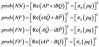
Hence, the referee observing the game state in the action basis sees each pure action state with probability given by
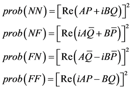 (2.10)
This result leads to the following definition:
Definition 2.1 Let G be the game described in Table1
Then the associated quantization
 with respect to the initial state ψ is the two player game in which each player’s
strategy space is the set of special unitary matrices, SU(2), and the quantum payoff
functions for Player I and Player II are defined as follows:
with respect to the initial state ψ is the two player game in which each player’s
strategy space is the set of special unitary matrices, SU(2), and the quantum payoff
functions for Player I and Player II are defined as follows:
 (2.11)
 (2.12)
As Equations (2.10) - (2.12) indicate, the use of SU(2) elements will prove impractical when one undertakes the important task of identifying potential quantum Nash equilibria of the game indicated in Table1 We will utilize the unit quaternions instead of the SU(2) elements. The unit quaternions turn out to be more efficient and convenient in simplifying a great deal of equilibrium calculations.
First, we begin with a brief review of the real division algebra of the quaternions which can be also found in [5] and [6] .
3. Quaternions
The quaternions, denoted by H, are a 4-dimensional normed division algebra over the real numbers. They are spanned by the identity element 1 and three imaginary units i, j, and k. These fundamental units satisfy the so-called Hamilton’s relation given by Equation (2.1). A general quaternion q has form
 (3.1)
(3.1)
where a, b, c, and d are real numbers. Addition and multiplication with quaternions
are polynomial, subject to Hamilton’s relation above. Multiplication with quaternions
is not commutative but the distributive law holds. When a = 0, that is, when , we call q a pure quaternion. Each quaternion
as above possesses a quaternionic conjugate
, we call q a pure quaternion. Each quaternion
as above possesses a quaternionic conjugate
 with
with . The real-valued norm (or length) on the
quaternions is defined by the formula
. The real-valued norm (or length) on the
quaternions is defined by the formula
 (3.2)
(3.2)
One can easily verify that the norm of a product of quaternions is the product of their norms, that is,
 (3.3)
(3.3)
Each non-zero quaternion possesses a non-zero inverse
 (3.4)
(3.4)
This establishes the set of non-zero quaternions as division algebra. Moreover, the set of unit quaternions
 (3.5)
(3.5)
forms a subgroup of H – {0} under quaternionic multiplication and can be thought as the unit 3-sphere S3 living in R4. In light of the discussion above, one can see that the set of non-zero quaternions forms a skew-field.
We can also express a general quaternion in the form
 where
where
 and
and
 are complex numbers. In this case, if
 , then quaternionic multiplication
is given by the map
, then quaternionic multiplication
is given by the map
 (3.6)
(3.6)
There are other identifications of S3 that are of interest to us beyond that of the unit quaternions, in particular the identification of S3 with the special unitary group of two-by-two complex matrices, SU(2). That is, those matrices with orthonormal columns and determinant 1. This group isomorphism is given by the map
 (3.7)
(3.7)
where the complex numbers
 and
and
 are subject to the normalization condition

For more details on real division algebras in general, and on quaternions in particular, the reader is referred to [7] [8] .
Unit Quaternions as Strategies
There are many isomorphisms between the group SU(2) of special unitary matrices and the group S3 of unit quaternions. We consider the following identifications.
Proposition 3.1.1 SU(2) and S3 are isomorphic as groups via the identifications
 (3.8)
(3.8)
and
 , (3.9)
where
 and A, B, P, Q are complex numbers such that

Proof: We prove that Equation (3.8) defines a group isomorphism. The proof that
Equation (3.9) is a group isomorphism is similar but omitted. Define the mapping
 by
by . First, we show that
 is a unit quaternion. For this, set
 Then
Then
 (3.10)
and has norm
 (3.11)
since the SU(2) element
 has the property that
 This shows that the image of an SU(2) element under the mapping
 is a unit quaternion.
Next, we show that the mapping
 is a group homomorphism. For this, let
 and
and
 be arbitrary elements of SU(2). Then, on one hand
 (3.12)
and on the other hand
 (3.13)
Hence,
 for all
 . It remains to show that
 is one-to-one and onto. Note that
 yields

This can happen if and only if
 that is,
 and
and
 Therefore,
 which proves that
 is one-to-one.
Finally, note that each unit quaternion
 has the SU(2) element
 , where
 , as a pre-image under
the map
, as a pre-image under
the map . Therefore,
 is onto. This completes the proof that
 is a group isomorphism. ■
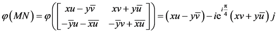
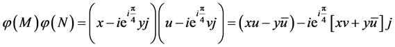
Now we take p and q as given in Equations (3.8) and (3.9) and compute the product
 (3.14)
This product can be also expressed as
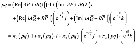 (3.15)
where

 and
and

To further simplify the product pq, we utilize the following straightforward identities
(1)

(2)

Therefore the expression for pq simplifies to
 (3.16)
Comparing Equations (2.10) and (3.16), we conclude that
 (3.17)
This result motivates the following definition.
Definition 3.1.2 Let G be the game depicted in Table1
Then the corresponding pure quantum game with respect to the initial state ψ,
 , is the two player game in which each player’s strategy
space is the set of unit quaternions with basis
, is the two player game in which each player’s strategy
space is the set of unit quaternions with basis
 and Player I’s and Player II’s payoff functions are given by
 (3.18)
We observe that the basis
 is an orthonormal basis of H. In practice, the players would love to use unit quaternions
that are linear combinations of the elements of the canonical basis of H,
is an orthonormal basis of H. In practice, the players would love to use unit quaternions
that are linear combinations of the elements of the canonical basis of H, . An easy exercise is to observe
that the basis change matrix from basis B1 to basis B0 is
. An easy exercise is to observe
that the basis change matrix from basis B1 to basis B0 is
 (3.19)
This matrix is unitary, therefore the basis change matrix from B0 to B1 is
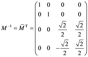 (3.20)
If the players employ unit quaternions based on 1, i, j, and k then the payoffs to Player I and Player II are
 (3.21)
 (3.22)
respectively, where xt and yt are taken from Table1 These results are summarized in the following definition.
Definition 3.1.3 Let G be the game depicted in Table1
Then the corresponding pure quantum game with respect to the initial state ψ,
 , is the two player game in which each player’s strategy
space is the set of unit quaternions with basis
, is the two player game in which each player’s strategy
space is the set of unit quaternions with basis
 and Player I’s and Player II’s payoff functions are given by Equations (3.21) and
(3.22), respectively.
and Player I’s and Player II’s payoff functions are given by Equations (3.21) and
(3.22), respectively.
We conclude this section with the observation that the map
 is onto as opposed to the map
 of Section 1. Indeed, for any probability distribution over the outcomes of the
game G described in Table 1,
of Section 1. Indeed, for any probability distribution over the outcomes of the
game G described in Table 1,
 ,there are unit quaternions p and q such that
 .
.
It is sufficient to choose p = 1 and .
.
4. Mixed Quantum Strategies
A mixed quantum strategy is a probability distribution over the set of unit quaternions.
While the consideration of the entire space of mixed quantum strategies remains a goal of a future work, the use of mixed quantum strategies supported on the canonical basis elements 1, i, j and k, that is, elements of the form
 ,
,
 and
and , (4.1)
has already established some interesting results.
Definition 4.1 Let G be the game depicted in Table1
Then the corresponding mixed quantum game with respect to the initial state ψ,
 , is the two player game in which each player’s strategy
space is the set of probability distributions over the unit quaternions and Player
i’s expected payoff function is
, is the two player game in which each player’s strategy
space is the set of probability distributions over the unit quaternions and Player
i’s expected payoff function is
 .
.
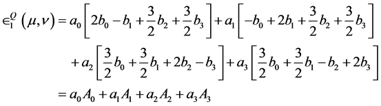
As we did in the game GQ, we will derive equations for the players’ expected
payoff functions in the game . For this, suppose Player I
uses the mixed quantum strategy
. For this, suppose Player I
uses the mixed quantum strategy
 (4.2)
(4.2)
and Player II uses the mixed quantum strategy
 (4.3)
(4.3)
Then the expected payoff to Player I is given by
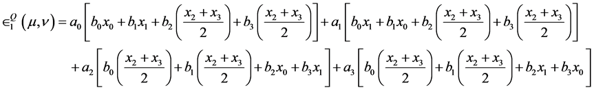 (4.4)
(4.4)
or, in matrix form
 (4.5)
(4.5)
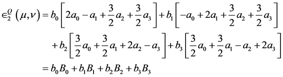
Player II’s expected payoff is derived in a similar manner, except that the letter x is replaced with the letter y.
We note here the similarities between the quantum expected payoff function in
 (Equation (4.5)) and the classical expected payoff function in Gmix (Equation
(1.6)).
(Equation (4.5)) and the classical expected payoff function in Gmix (Equation
(1.6)).
Note that we can also express Equation (4.4) in the form
 , (4.6)
and similarly
 . (4.7)
Equation (4.7) is the expected quantum payoff function for Player II. We will refer to the coefficients at and bt as the frequencies and the numbers At and Bt as the returns.
5. Application
As an application of the theory discussed in the previous sections, we consider a variant of the game of Chicken with bimatrix given by Table2
In the Game of Chicken, the expected payoff to Player I is given by
 (5.1)
(5.1)
with corresponding best reply correspondence R1: [0, 1]→[0,1] given by
 (5.2)
(5.2)
Similarly, Player II’s expected payoff function is given by
 (5.3)
(5.3)
with corresponding best reply correspondenceR2 : [0, 1]→[0,1] given by
 (5.4)
(5.4)
The reaction curves that represent these correspondences are shown in Figure 1, with the dashed lines for Player I’s reaction curve and the solid lines for Player II’s reaction curve.
It is well known that in any variant of the game of chicken there are always three classical equilibria, two in pure strategies and one in mixed strategies. Nash equilibria occur where the reaction curves intersect. From Figure 1, one can see that the classical pure equilibria are (p = 0, q = 1) and (p = 1, q = 0) or, equivalently, the pure strategy pairs (s2, t1) and (s1, t2) with corresponding payoffs (3, 0) and (0, 3) to the players, respectively.
The equilibrium in mixed strategies is the pair . This equilibrium pays
out each player an expected payoff of 1.
. This equilibrium pays
out each player an expected payoff of 1.
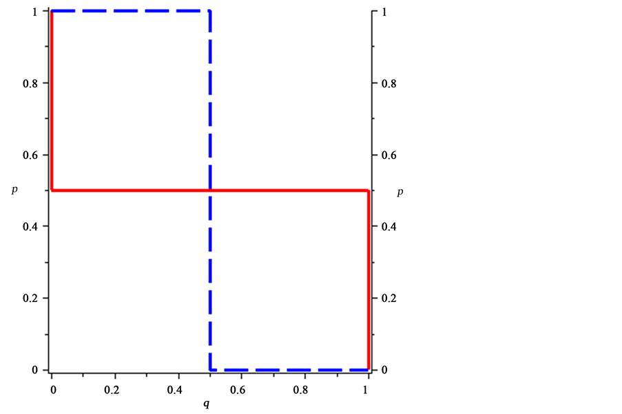
Figure 1. Reaction curves in the game of chicken.
However, in contrast to the classical situation, we find, using best response analysis, that the quantized version possesses many Nash equilibria.
5.1. Equilibria of Type (Pure, Pure)
There are four equilibria where each player employs a pure quantum strategy represented by a canonical quaternionic basis element.
Proposition 5.1 The Game of Chicken described in Table 2 admits the following Nash equilibria in pure quantum strategies:
 (5.5)
(5.5)
 (5.6)
(5.6)
 (5.7)
(5.7)
 (5.8)
(5.8)
Moreover, these equilibria pay out each player an expected payoff of 2.
Proof: If Players I and II employ the mixed quantum strategies
 and
and
 , respectively, then, by Equation (4.4), the expected
payoffs to the players are
, respectively, then, by Equation (4.4), the expected
payoffs to the players are
 (5.9)
(5.9)
and
Table 2 . Game of chicken.
 (5.10)
Suppose that A0 is the largest return. Then Player I will choose a µ
that concentrates all the frequencies on A0, that is
 or µ=1. Therefore, Player II’s expected payoff becomes
 (5.11)
It is clear that Player II’s expected payoff is maximal when he or she responds
with a ν that concentrates all the frequencies on the largest return 2, that is,
 and therefore ν = 1 is the best reply to Player
I’s choice of µ = 1. Now suppose that Player II selects the unit quaternion
ν = 1 as a strategy. Then Player I’s expected payoff becomes
and therefore ν = 1 is the best reply to Player
I’s choice of µ = 1. Now suppose that Player II selects the unit quaternion
ν = 1 as a strategy. Then Player I’s expected payoff becomes
 (5.12)
Then Player I’s best response will be to select µ=1.Therefore, the pure quantum
strategic pair
 is a Nash equilibrium with the expected payoff of
 to the players. In a similar manner, when At, t = 1, 2, 3 is maximal,
one verifies that the pure quantum strategic pairs
to the players. In a similar manner, when At, t = 1, 2, 3 is maximal,
one verifies that the pure quantum strategic pairs
 and
and
 are Nash equilibria with an expected payoff of 2 to each player.
Equilibria in mixed quantum strategies occur when two or more returns are equal and maximal.
5.2. Equilibria of Type (Mix of 2, Mix of 2)
We begin with the situation where two returns are equal and maximal.
Proposition 5.2 The Game of Chicken admits the following Nash equilibria in mixed quantum strategies:
 with
with
 (5.13)
 (5.14)
 (5.15)
 (5.16)
 (5.17)
 with
with
 (5.18)
Moreover, all these equilibria pay out each player an expected payoff of 7/4, except the equilibria given by (5.13) and (5.18) which pay out each player an expected payoff of 1.5.
Proof: We begin by proving that the strategic pair given in Equation (5.13) is a
Nash equilibrium. For this, suppose that the returns A0 and A1
are equal and maximal. Then, Player I will select that is,
 and
and . Therefore, Player
II’s expected payoff becomes
. Therefore, Player
II’s expected payoff becomes
 (5.19)
To determine the largest return, we graph
 and
and
 against the frequency a0, see Figure 2.
From the graphs, we see that Player II will respond with v = 1, i, j, or k when . However, from Proposition 5.1, we know that a
best reply to v = 1, i, j, or k is μ = 1, i, j, or k, respectively. So we disregard
the cases
. However, from Proposition 5.1, we know that a
best reply to v = 1, i, j, or k is μ = 1, i, j, or k, respectively. So we disregard
the cases
 and
and . When
 , the largest returns
are
, the largest returns
are . HencePlayer II will respond with

Now suppose that Player 2 selects the mixed quantum strategy
 together with the condition that
 . Then, Player I’s expected
payoff becomes
. Then, Player I’s expected
payoff becomes
 (5.20)
Figure 3 shows the graphs of the returns
 and
and
 against the frequency b2.
From the graphs, we see that Player I will respond with µ = 1, i, j, or k
when . This contradicts the condition
 . So we disregard the
cases
. So we disregard the
cases
 and
and . When
 , the largest returns
are
, the largest returns
are . Hence, Player I will respond with

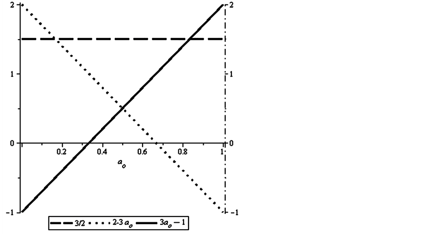
Figure 2. Graphs of the returns B0, B1, B2 and B3.
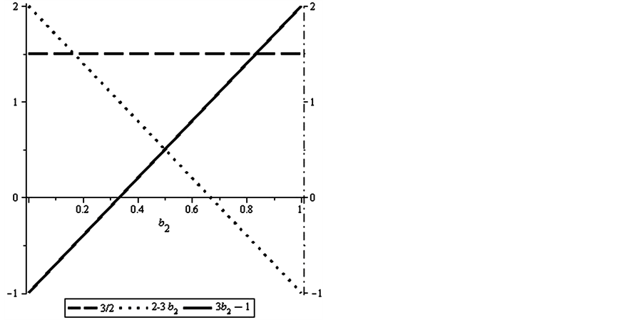
Figure 3. Graphs of the returns A0, A1, A2 and A3.
Therefore, we have a family of equilibria given by the strategic pair
 with the constraints that
 and
and . This family of equilibria pays out each player
an expected payoff of
. This family of equilibria pays out each player
an expected payoff of
 .
.
In a similar manner, One verifies that the strategic pairs given in (5.14) - (5.18) are Nash equilibria.
5.3. Equilibria of Type (Mix of 3, Mix of 3)
When three returns are maximal and equal, we obtain four cases to study. For this particular game, it turns out that there are no equilibria of type mix of 3 against mix of 3.
5.4. All the Returns Are Equal
Proposition 5.3 The mixed quantum strategic pair

is a Nash equilibrium with expected payoffs to the players given by .
.
Proof: When all the returns are equal, Player I is indifferent between all his/her mixed strategies and, therefore, can select any probability distribution over the returns A0, A1, A2, and A3. The equations A0= A1 = A2 = A3 yield the system of linear equations
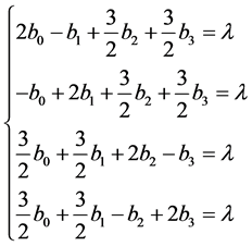 , (5.21)
where λ is a fixed real number. This system has the unique solution

Since
 we obtain

Now suppose Player II uses the mixed quantum strategy
 Then Player I’s expected payoff becomes
 Hence Player I is indifferent between all his/her probability distributions. In
particular, he/she can respond with
Hence Player I is indifferent between all his/her probability distributions. In
particular, he/she can respond with
 Therefore, the mixed quantum strategic pair
 is a Nash equilibrium with expected payoffs to the players given by
 .
.
6. Conclusions
It often happens that the players’ reaction curves cross several times as is the case in the game of Chicken. The classical version of the game of Chicken has three equilibria. Which of these should be selected? Only the equilibrium in mixed strategies that pays out each player a payoff of 1 makes sense for rational players, as the selection of one of the remaining two classical equilibria will result in one of the players being worse off. We, therefore, observe that the quantum payoffs are all equal or superior to the classical payoff (1, 1) that is desired by both players.
Moreover, comparing our findings to known results, we observe that the strategic
pair
 is also an equilibrium in Landsburg’s quantized game of Chicken with expected payoffs
of (2.5, 1) to the players [4] . Recall that, in
our game, the payoff to each player at this equilibrium is 7/4. Thus, Player II
is better off playing Chicken when it is quantized via our initial state.
is also an equilibrium in Landsburg’s quantized game of Chicken with expected payoffs
of (2.5, 1) to the players [4] . Recall that, in
our game, the payoff to each player at this equilibrium is 7/4. Thus, Player II
is better off playing Chicken when it is quantized via our initial state.
The groundwork for a parallel extension of this work to three player, two strategy games can be found in [9] and [10] . A future direction of this work is the complete classification of potential Nash equilibria in three player, two strategy quantum games.
Acknowledgements
The authors would like to thank the referees for some valuable comments and helpful suggestions.
References
[1] Eisert, J., Wilkens, M. and Lewenstein, M. (1999) Quantum Games and Quantum Strategies. Physical Review Letters, 83, 3077-3080. http://dx.doi.org/10.1103/PhysRevLett.83.3077
[2] Bleiler, S.A. (2008) A Formalism for Quantum Games and an Application. Proceedings to the 9th International Pure Math Conference, Islamabad.
[3] Nash, J. (1950) Equilibrium Points in N-Person Games. Proceedings of the National Academy of Sciences of the United States, 36, 48-49. http://dx.doi.org/10.1073/pnas.36.1.48
[4] Landsburg, S. (2011) Nash Equilibria in Quantum Games. Proceedings of the American Mathematical Society, 139, 4423-4434. http://dx.doi.org/10.1090/S0002-9939-2011-10838-4
[5] Ahmed, A. (2013) Quantum Games and Quaternionic Strategies. Quantum Information Processing, 12, 2701-2720. http://dx.doi.org/10.1007/s11128-013-0553-5
[6] Ahmed, A. (2013) Equilibria in Quantum Three-Player Dilemma Game. British Journal of Mathematics & Computer Science, 3, 195-208. http://dx.doi.org/10.1007/s11128-013-0553-5
[7] Baez, J. (2002) The Octonions. Bulletin of the American Mathematical Society, 39, 145-205. http://dx.doi.org/10.1090/S0273-0979-01-00934-X
[8] Conway, J.H. and Smith, D.A. (2003) On Quaternions and Octonions. A. K. Peters, Wellesley, Massachusetts.
[9] Ahmed, A. (2011) On Quaternions, Octonions, and the Quantization of Games: A Text on Quantum Games. Lambert Academic Publishing, Saarbrücken.
[10] Ahmed, A.O., Bleiler, S.A. and Khan, F.S. (2010) Octonionization of Three-Player, Two-Strategy Maximally Entangled Quantum Games. International Journal of Quantum Information, 8, 411-434. http://dx.doi.org/10.1142/S0219749910006344