Advances in Pure Mathematics
Vol.4 No.4(2014), Article ID:45189,9 pages DOI:10.4236/apm.2014.44020
Interval Analytic Method in Existence Result for Hyperbolic Partial Differential Equation
Peter O. Arawomo
Department of Mathematics, University of Ibadan, Ibadan, Nigeria
Email: womopeter@gmail.com
Copyright © 2014 by author and Scientific Research Publishing Inc.
This work is licensed under the Creative Commons Attribution International License (CC BY).
http://creativecommons.org/licenses/by/4.0/


Received 2 January 2014; revised 2 February 2014; accepted 15 February 2014
ABSTRACT
Without the usual assumption of monotonicity, we establish some results on the theory of hyperbolic differential inequalities which enable us to produce a majorising interval function for the solution of the hyperbolic initial value problem. Using this function, a variation of parameters formula and interval iterative technique, the existence of solution to the problem is established.
Keywords:Interval Functions, Interval Majorant, Interval Extension, Interval Operator, Nested Sequence

1. Introduction
In this paper, we utilize interval analytic methods in the investigation of the existence of solution of the hyperbolic partial differential equation
 (1.1)
(1.1)
with characteristic initial values
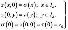 (1.2)
(1.2)
prescribed in a two-dimensional rectangle  where
where 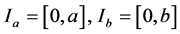
 and
and

 ,
, 
 and
and  where
where  means that z is continuous on
  and possesses continuous partial derivatives
  on
on 
Without the assumption of monotonicity on the function  we establish some results on the theory of hyperbolic differential inequalities which enable us to produce a majorizing interval function for the solution of the equation. With the use of a variation of parameters formula used in [1] and theorem 5.7 of [2] on interval iterative technique we generate a nested sequence of interval functions which converges to an interval solution. This interval solution is thus a majorant of the solution of the equation and it coincides with the real valued solution if it is degenerate. Similar interval methods had earlier been used by some authors in [3] -[7] for solution to differential equation but not for hyperbolic initial value problems. The result in this paper generalizes those of [1] [8] as the monotonicity condition imposed on the function
  is not in any way necessary.
The basic results in interval analysis used in this work are found in [2] [6] [7] [9] -[13] for readers who may not be familiar with them.
2. Differential Inequalities and Majorisation of Solution
Definition 2.1: A function  is said to be an upper solution of the hyperbolic initial value problem (1.1) and (1.2) on
  if
if


 .
.
Definition 2.2: A function  is said to be a lower solution of the hyperbolic initial value problem (1.1) and (1.2) on
  if the reversed inequalities hold true with
  in place of
  in the specified intervals.
Next, we shall consider some results concerning the upper and lower solutions of Equation (1.1) and conditions (1.2).
Theorem 2.1: Suppose that  and
and
 (2.1)
(2.1)
 (2.2)
(2.2)
 (2.3)
(2.3)
Then we have
 (2.4)
(2.4)
where the inequality is componentwise.
Proof: We shall establish this theorem by contradiction. From assumption (2.3) we see clearly that the theorem is true for the point (0,0) on 
Suppose that inequality (2.4) is not true at a point  and assume that
 (2.5)
(2.5)
then by assumption (2.3)  and
and  cannot both be zero.
Let  be such that
  then
then  and so

Thus, we have, for  (or
(or ),
),
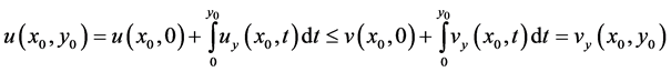
and this contradicts assumption (2.5).
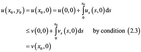
If  then
then  (or vice-versa) and for
  we have
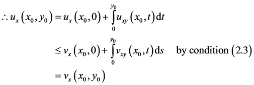
If  and
and  a similar argument can be advanced to obtain
  Hence,

and this is still a contradiction to our earlier assumption (2.5).
Suppose instead that
 (2.6)
(2.6)
Then  otherwise condition (2.3) would immediately give the required contradiction.
Now for  let
let  such that
 , we have
  so
so

This contradicts assumptions (2.6).
Similarly, if we assume that , we would also arrive at a contradiction. At
  and
and  left hand derivatives are used to obtain the result.
Hence, we conclude that, the assertion (2.4) holds true on  and this proves the theorem.
Theorem 2.2: Let  and
and  be functions defined on
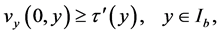
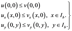
  which satisfy assumptions (2.1), (2.2) and (2.3) of Theorem 2.1. Suppose in addition that they satisfy the following conditions,
 (2.7)
(2.7)
Then the solution  of problem (1.1) and (1.2) together with its derivatives
  satisfy

On the rectangle,  , where the inclusion is componentwise.
Proof: Notice that the lower endpoints of the intervals in Equation (2.7) satisfy assumption (2.3) of Theorem 2.1 when  is replaced by
 . Therefore
  and
and  satisfy the hypothesis of Theorem 2.1 and hence
 (2.8)
(2.8)
Similarly, replacing  by
by  in assumption (2.3) we obtain the upper endpoints of the intervals in conditions (2.7) and so by Theorem 2.1 we also have
 (2.9)
(2.9)
Combining inequalities (2.8) and (2.9) we have the desired result.
3. Construction and Existence of Solution
Our purpose in this section is to establish the existence of solution to the problem (1.1) satisfying initial values (1.2) by means of interval analytic method. To this end an integral operator is constructed, the solution of the resulting operator equation is equivalent to the solution of the initial value problem under consideration. An interval extension of this operator is then used to generate a sequence of interval functions which converges to the required solution.
Let  be such that
  on
on  and a function
  , defined by
 (3.1)
(3.1)
where  is the function in Equation (1.1) and
  is a constant suitably chosen such that
  Clearly it can be seen that
  is continuous on
With this new function , Equation (1.1) becomes
 (3.2)
(3.2)
By using the variation of constant formula of Lemma 4.1 in [1] , we obtain the solution of Equation (3.2), satisfying initial values (1.2) as:

Differentiating with respect to , we obtain

and similarly by differentiating with respect to  we obtain

Eliminating the derivatives  and
and  by introducing the function
  and
and  into the integro-differential equations we obtain the system of integral equations
 (3.3)
(3.3)
 (3.4)
(3.4)
 (3.5)
(3.5)
which is equivalent to the problem (3.2) and initial values (1.2).
Denoting the right hand side of these integral equations by  and
and  respectively, we have the following:
 (3.6)
(3.6)
With these we prove the following result.
Lemma 3.1: Let  and
and  satisfy conditions (2.7) of Theorem 2.2. Suppose that for functions
  with
with 
 on
on , we have
 (3.7)
(3.7)
where  is the constant appearing in Equation (3.1). Then the following hold true.
 (3.8)
(3.8)
for all 
Proof: We first consider the lower endpoints of the inclusions and differentiating we have, from Equation (3.3)

differentiating again with respect to  we obtain
This, by Equation (3.1) and assumption (3.7), gives

Similarly by differentiating Equation (3.3) with respect to , we obtain

By conditions (2.1) and (3.7) we have  for
for  and
and  for
for  From these we see that
  satisfies the assumptions of Lemma 4.2 of [1] since
Thus


It could similarly be proved that

and

Hence the lemma is established.
Theorem 3.1: Let the functions  satisfy conditions (2.7). Suppose that the function
  is such that

and
 for function
  satisfying

and , constant, suitably chosen in Equation (3.1).
Then there exists a convergent nested sequence of interval functions  such that the unique solution
  of Equations (1.1) and (1.2) satisfies

with ,
,  degenerate where the initial interval
  is given by

Proof: From the construction earlier considered, we see that any solution of Equation (1.1) which satisfies condition (1.2) solves the integral Equation (3.3). Conversely if  solves the integral Equation (3.3) we have that

which by Equations (3.1) and (3.6) gives
with
 .
.
and these imply that  again solves the Equation (1.1) and satisfies condition (1.2). Therefore, we shall seek the solution of the integral equation given by (3.3) which is transformed to the operator equation

Let  be an interval function defined on
  such that
  for
for  and the interval function
  an interval extension of the function
  defined in Equation (3.1). Then the interval integral operator
  defined by

is an interval majorant of .
.
Then the problem reduces to solving the interval operator equation

However to determine  we need to also determine
  and
and  which are respectively interval extensions to the function
  and
and . This is done by solving the interval operator equations
With  and
and  defined respectively by

and

which majorise the real operators  and
and  respectively.
Define the sequences  by
by
 with
with

 with
with
 and
and
 with
with

We have the sequence  as required.
We shall show that  convergences to a limit. But this can only be so if the sequence
  and
and  also converge.
By Theorem 5.7 of [2] , these sequences converge if

 and
and

Now for

by the first inclusion of Equation (3.8). Hence

Similarly we have by the result given in Equation (3.8) of Lemma 3.1

and

Since these initial intervals satisfy the hypothesis of Theorem 5.7 of [2] , the result of the theorem implies that  and
and  converge as sequences and are equally nested. Furthermore, the solution
  of Equation (1.1) satisfying condition (1.2) belongs to the limit function
  of the sequence
  that is,

and this proves the theorem.
Lemma 3.2: Assume that the functions  satisfy conditions (2.7) and in addition they also satisfy conditions (2.1) and (2.2). Suppose further that the function f appearing on the right hand side of Equation (1.1) satisfies:
 (3.9)
(3.9)
whenever the functions  and
and  are such that

for constant  suitably chosen. Then we have
 (3.10)
for any function  satisfying

Proof: From inequality (2.1) we have

Since

From inequality (3.9) we have

and so

which is the first inequality in (3.7).
Also from inequality (2.2) we have

and using inequality (3.9) we have

Therefore

which also is the second inequality in (3.7). Since all the other conditions of Lemma 3.1 are also satisfied, the proof of this lemma follows as for Lemma 3.1 to obtain the desired result.
Remark 3.1: If  in inequality (3.9) then we have

for  and this implies that
  is monotone increasing in its domain of definition. Therefore the result of lemma 3.2 also holds for a monotone function
Theorem 3.2: Suppose that the function  satisfies conditions (2.1), (2.2) and (2.7). If in addition the function
  appearing in Equation (1.1) satisfies

whenever

for some constant , suitably chosen.
Then there exists a nested sequence of interval function  with each term majorising the unique solution
  of Equation (1.1) satisfying condition (1.2) such that the limit
  of this sequence also contains
 , that is,

Proof: As it has been shown in the proof of Lemma 3.2, the conditions prescribed in this theorem can equally be linked with those of Theorem 3.1. Therefore the proof can be established in a manner similar to that of Theorem 3.1.
References
- Lakshmikantham, V. and Pandit, S.G. (1985) The Method of Upper and Lower Solution and Hyperbolic Partial Differential Equations. Journal of Mathematical Analysis and Applications, 105, 466-477. http://dx.doi.org/10.1016/0022-247X(85)90062-9
- Moore, R.E. (1979) Methods and Application of Interval Analysis. SIAM (Studies in Applied and Numerical Mathematics), Philadelphia. http://dx.doi.org/10.1137/1.9781611970906
- Arawomo, P.O. and Akinyele, O. (2002) An Interval Analytic Method in Constructive Existence Result for Initial Value Problems. Dynamic Systems and Applications, 11, 545-556.
- Chan, C.Y. and Vatsala, A.S. (1990) Method of Upper and Lower Solution and Interval Method for Semilinear EulerPision-Darboux Equations. Journal of Mathematical Analysis and Applications, 150, 378-381. http://dx.doi.org/10.1016/0022-247X(90)90110-2
- Lakshmikantham, V. and Swansundaran, S. (1987) Interval Method for 1st Order Differential Equations. Applied Mathematics and Computation, 23, 1-5. http://dx.doi.org/10.1016/0096-3003(87)90052-X
- Moore, R.E. (1984) Upper and Lower Bounds on Solutions of Differential, Integral Equations without Using Monotonicity, Convexity or Maximum Principle., In: Vichnevetsky, R. and Stepheman, R., Eds., Advances in Computer Methods for Partial Differential Equations, IMACS, 458-461.
- Moore, R.E. (1984) A Survey of Interval Methods for Differential Equations. Proceedings of 23rd Conference on Decision and Control, Las Vegas, 12-14 December 1984, 1529-1535.
- Walter, W. (1970) Differential and Integral Inequalities. Springer-Verlag, Berlin, Heidelberg. http://dx.doi.org/10.1007/978-3-642-86405-6
- Caprani, O. and Madsen, K. (1975) Contraction Mappings in Interval Analysis. BIT Numerical Mathematics, 15, 362- 366. http://dx.doi.org/10.1007/BF01931673
- Moore, R.E. (1977) A Test for Existence of Solution to Nonlinear Systems. SIAM Journal on Numerical Analysis, 14, 611-615.
- Moore, R.E. (1978) Bounding Sets in Function Spaces with Application to Nonlinear Operator Equations. SIAM Review, 20, 492-512.
- Rall, L.B. (1983) Mean-Value and Taylor Forms in Interval Analysis. SIAM Journal on Mathematical Analysis, 14, 223-238.
- Rall, L.B. (1982) Integration of Interval Functions II, the Finite Case. SIAM Journal on Mathematical Analysis, 13, 690-698.