ABSTRACT

We prove some value-distribution results for a class of L-functions with rational moving targets. The class contains Selberg class, as well as the Riemann-zeta function.

1. Introduction

We define the class to be the collection of functions

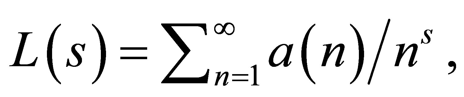satisfying Ramanujan hypothesisAnalytic continuation and Functional equation. We also denote the degree of a function by which is a non-negative real number. We refer the reader to Chapter six of [1] for a complete definitions. Obviously, the class contains the Selberg class. Also every function in the class is an -function and the Riemann-zeta function is in the class. In this paper, we prove a value-distribution theorem for the class with rational moving targets. The theorem generalizes the value-distribution results in Chapter seven of [1] from fixed targets to moving targets.

Theorem. Assume that and is a rational function with. Let the roots of the equation be denoted by. Then

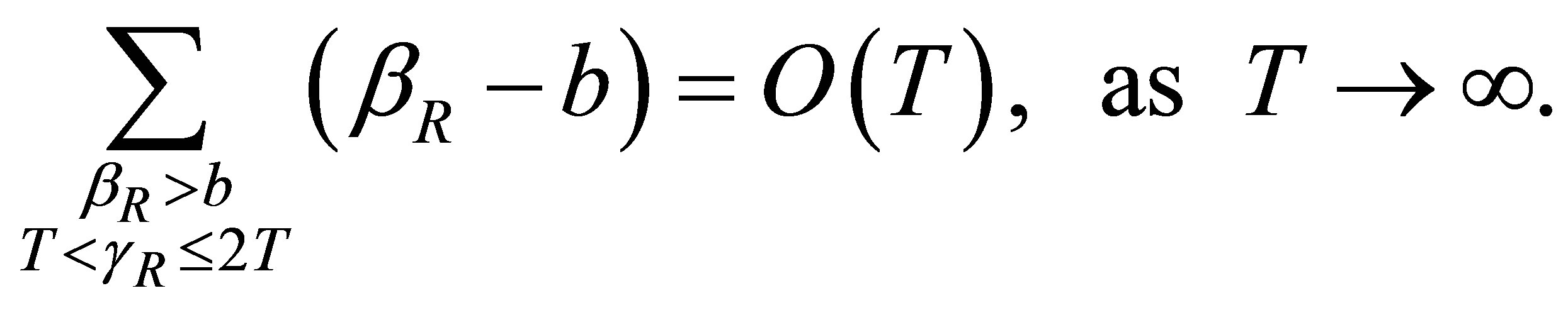
(I) For any,

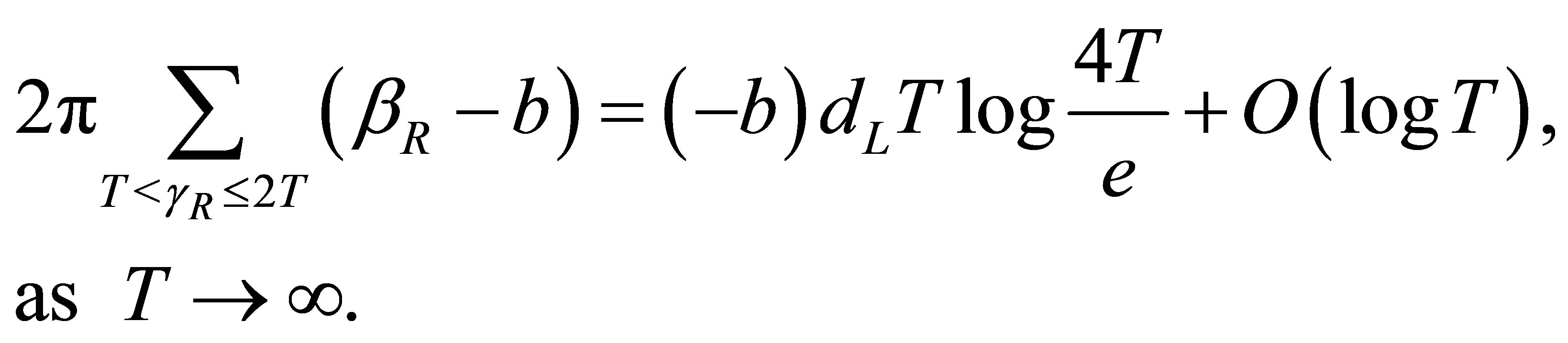
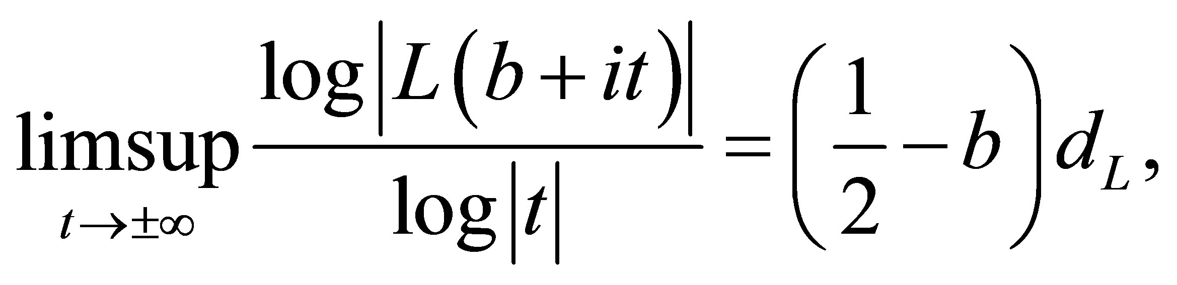
(II) For sufficiently large negative,

Proof of (I). It is known that if, then

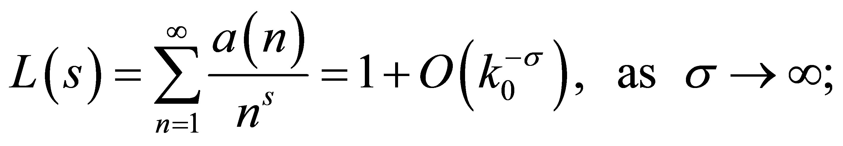
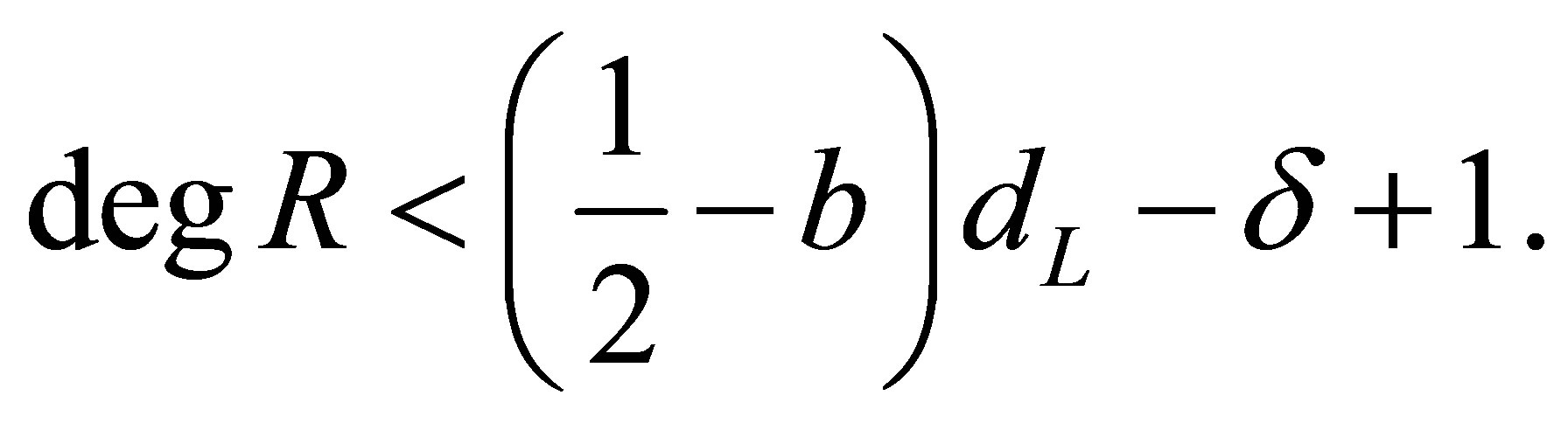
where is the index of the first non-zero term of the sequence of, with. Since, there exists such that for. It follows that for all real part of zeros of the function. We set where the degrees of are, respectively; and define

Thus, there is such that is analytic in the region since is a meromorphic function in with the only pole at. We apply Littlewood’s argument principle [3] to in the rectangl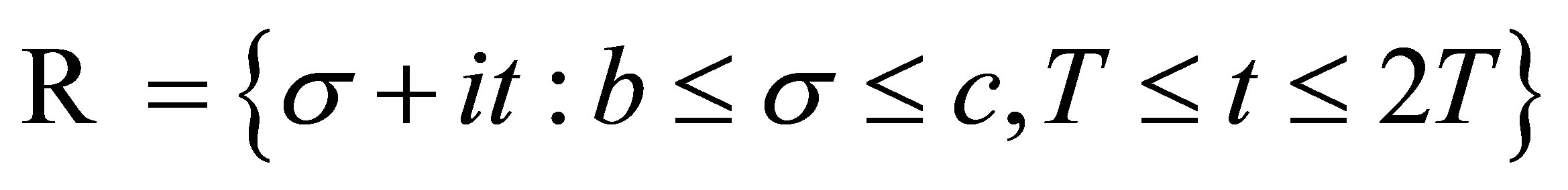e where are parameters satisfying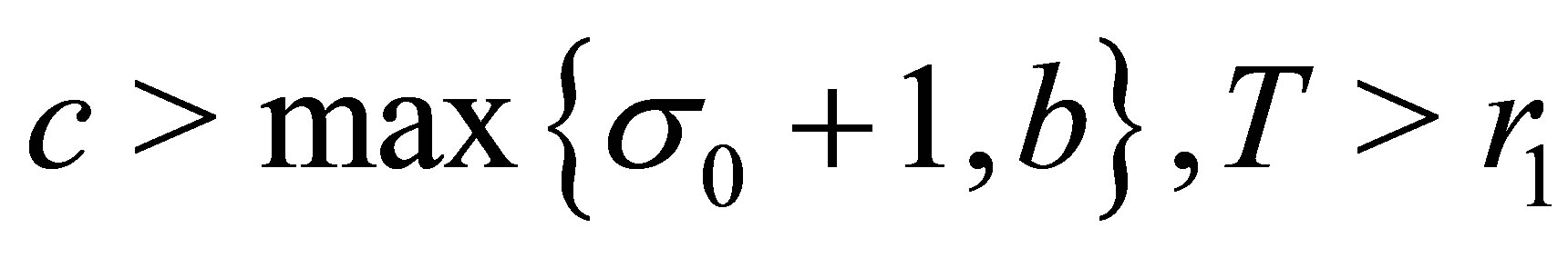. Thus,

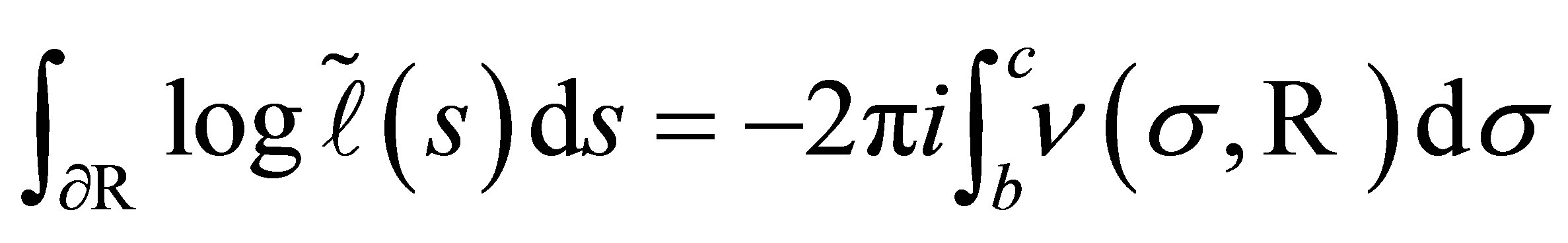
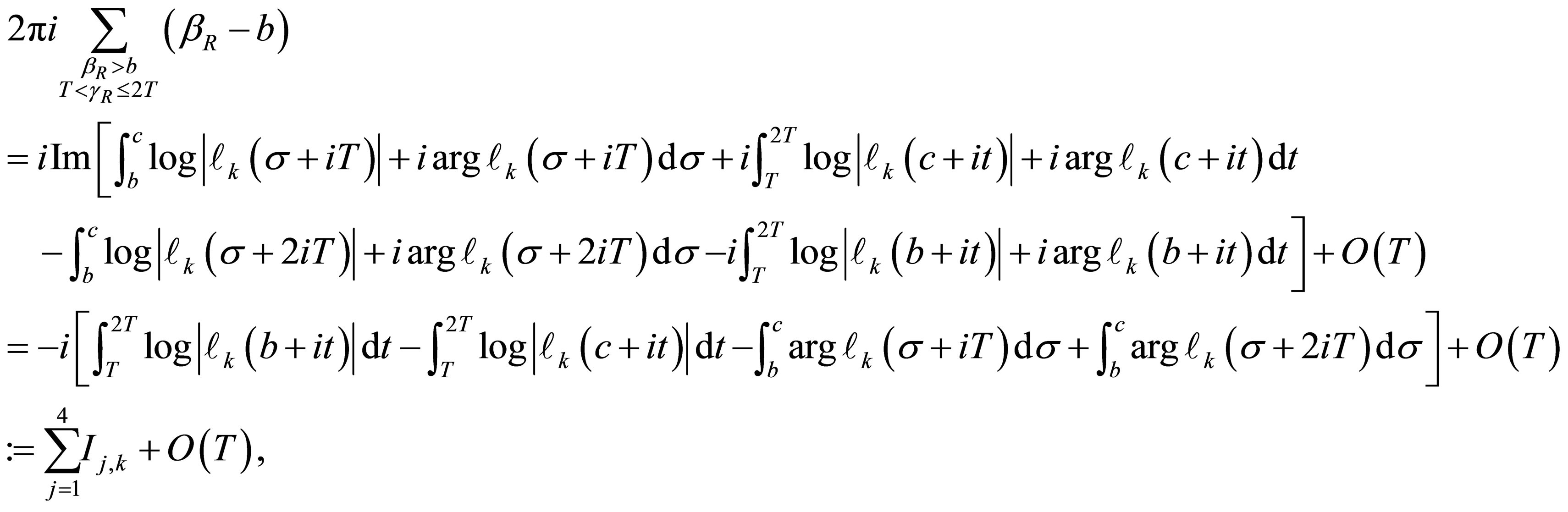
where the given logarithm is defined as in Littlewood’s argument principle [3]. To prove our result, however, we first decompose our auxiliary function by

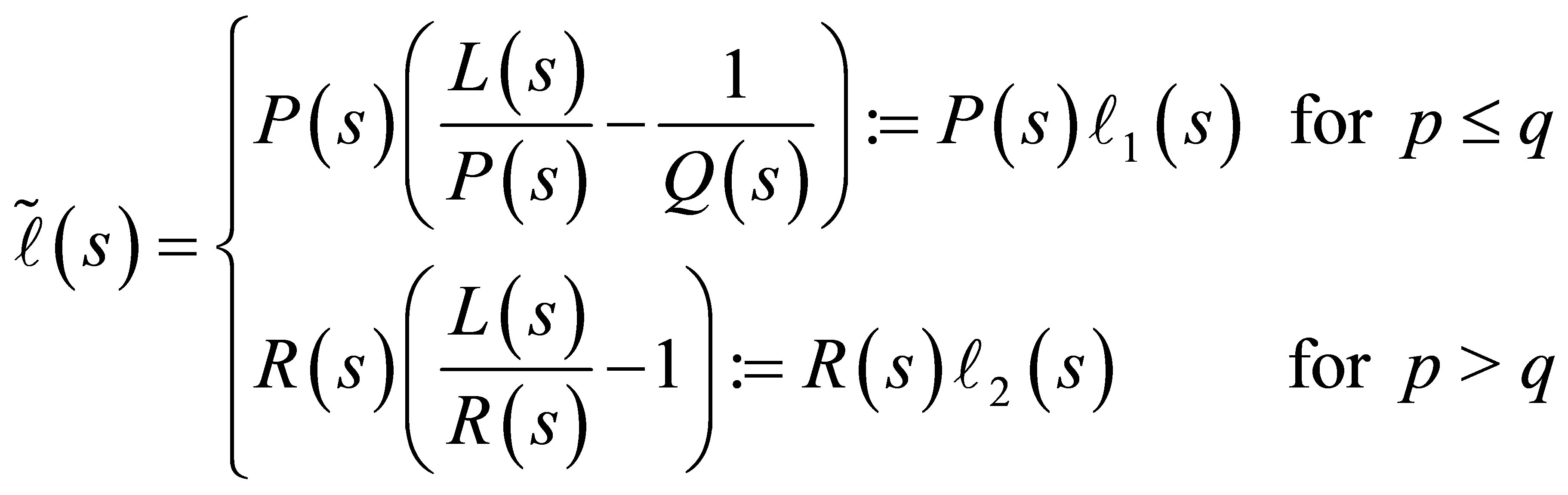(1)

Without loss of generality, we may assume that whenever since we can always write 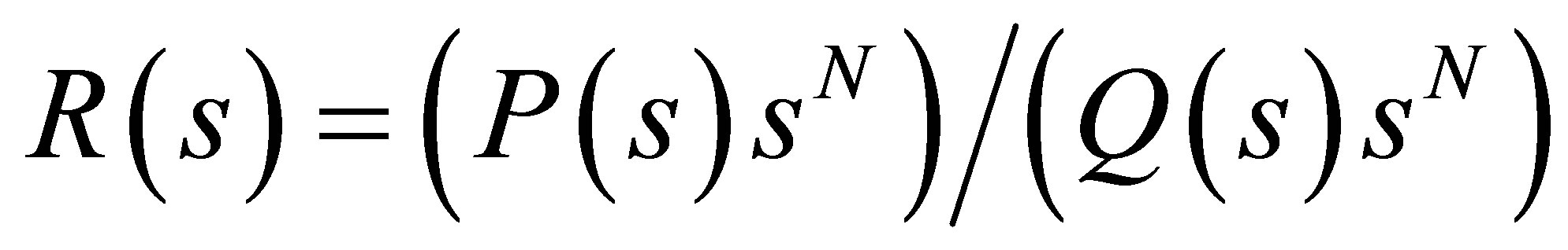for due to our choice of the parameters which define the rectangle. However, the modification will guarantee in the case of that exhibit polynomial growth, which is necessary for our proof. In the case of, already exhibits polynomial growth, and no such adjustment is necessary. We now integrate the logarithm of to get

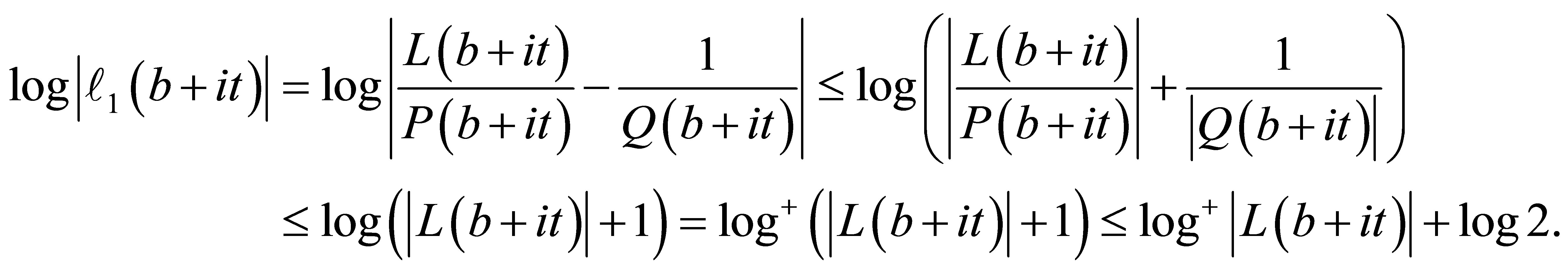
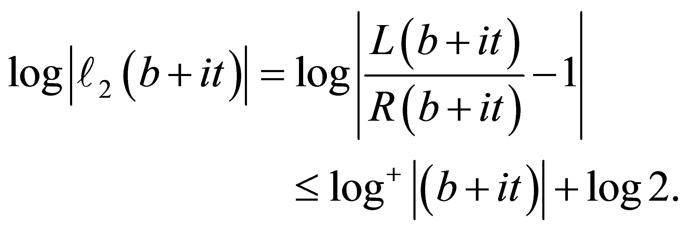
where the terms are the integrals of the maximum contribution from writing as a sum of logarithms. By our choice of, both and are analytic in Hence, Cauchy’s Theorem gives

(2)

To connect this integral with Littlewood’s argument principle [3], we note that the definition of guarantees that

(3)

In light of (2) and because the quantity given in (3) is imaginary-valued, we get for

(4)

for instance.

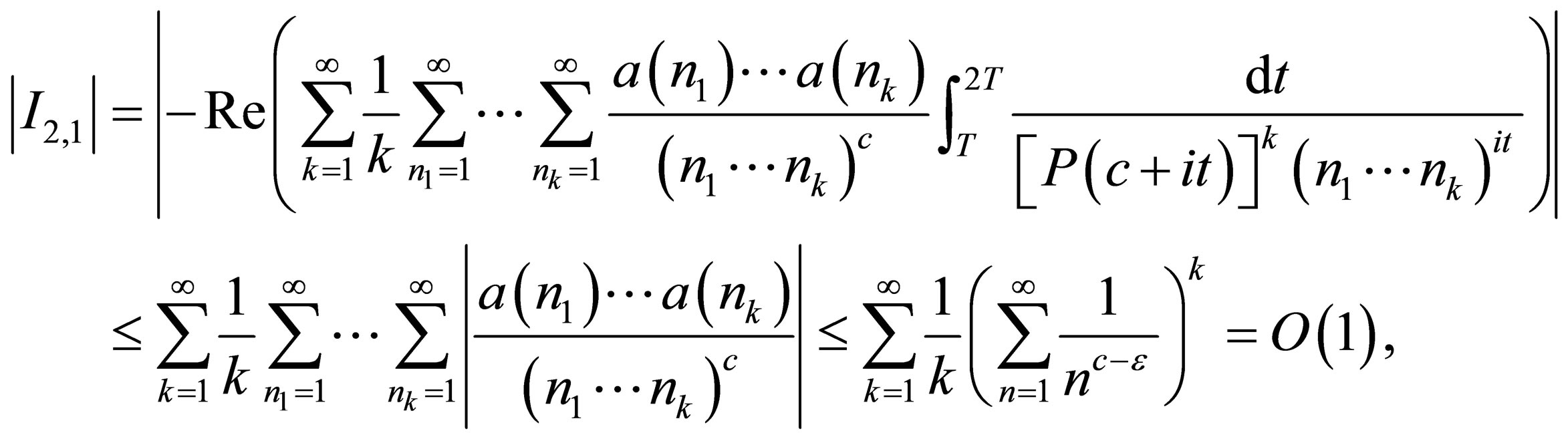
We now estimate. For large enough, we have for (since),

Then for large enough, , we find in a similar fashion that

Since we have the same estimate for, we find that

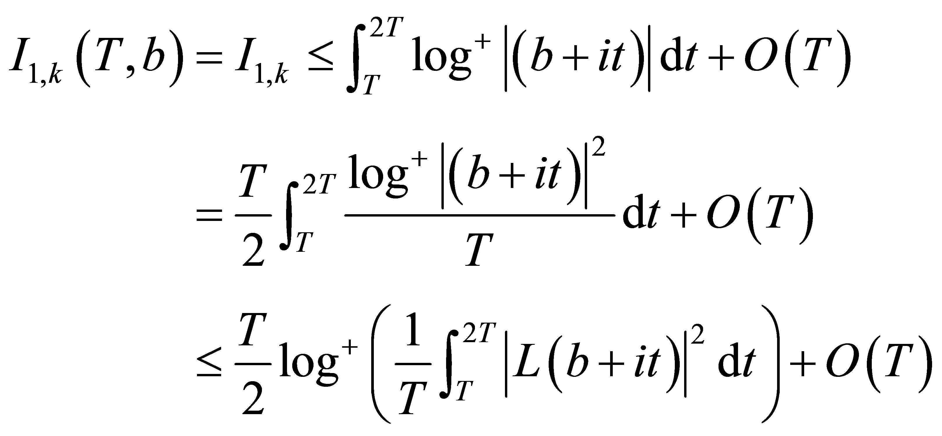
where the final bound follows from Jensen’s inequality. It is known [2] that for,

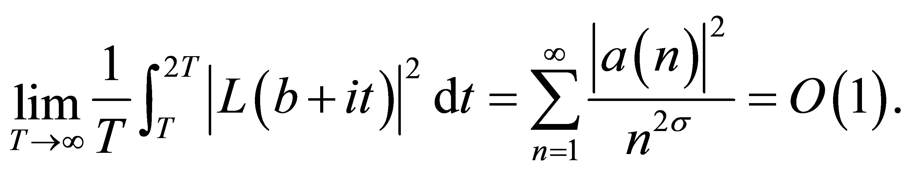
Hence, 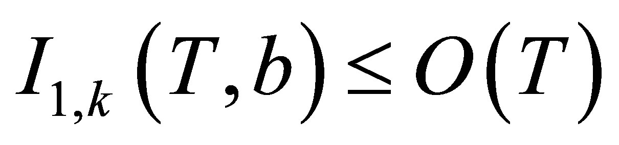uniformly in .

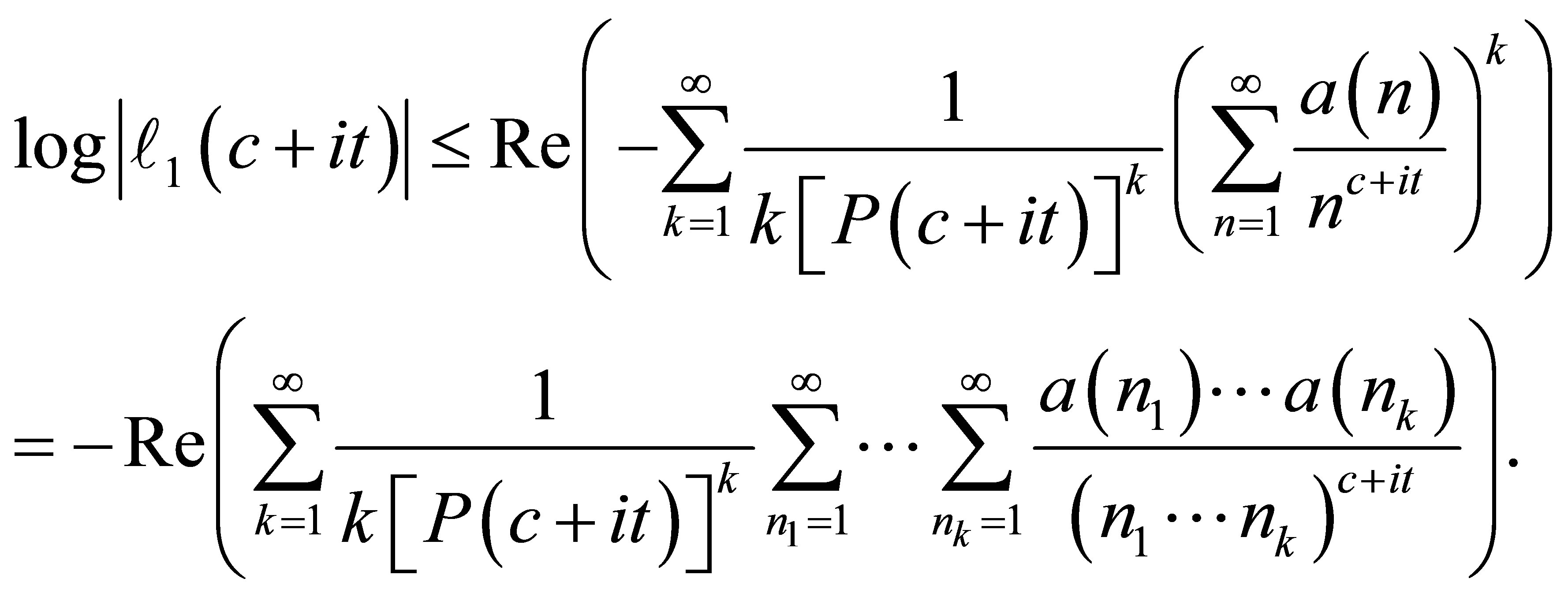
We next move to estimate. For sufficiently large positive real number, we have

(5)

so

since. Furthermore,

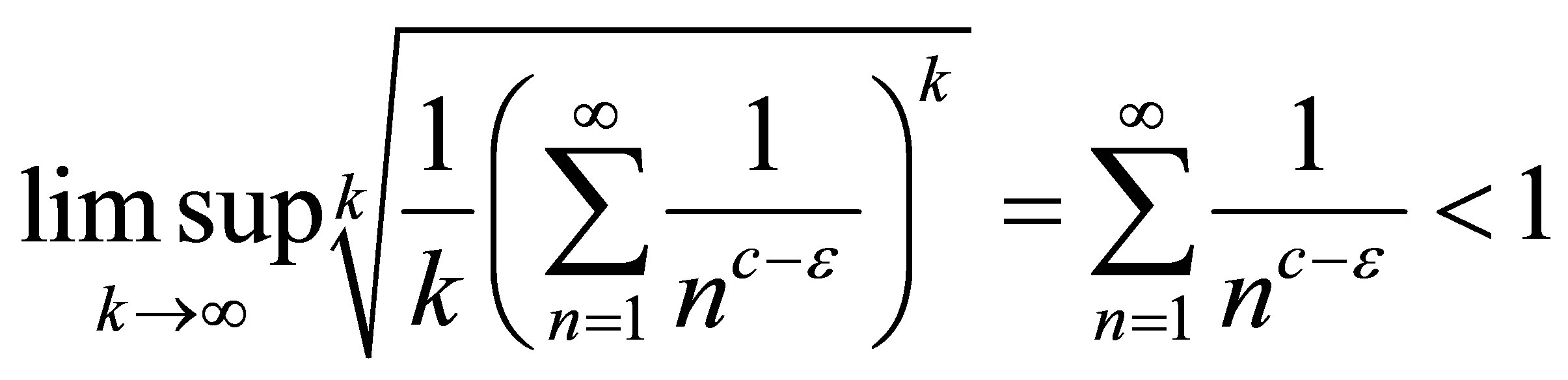
Since we may take large enough so that

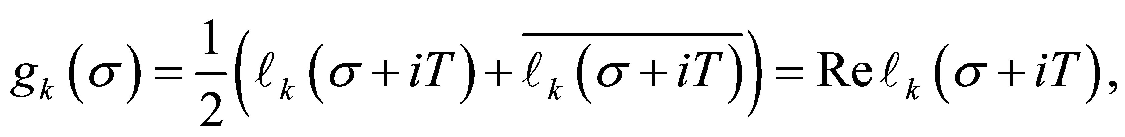
, we may write using a Taylor series expansion in the rectangle. For, we have after taking real parts that

We now observe that for sufficiently large T and some constant M we have

for and

for sufficiently large. In light of these bounds and the definition of, we have (6)

where the last equality holds because could be sufficiently large. Replacing by in the above computations, we see analogously that.

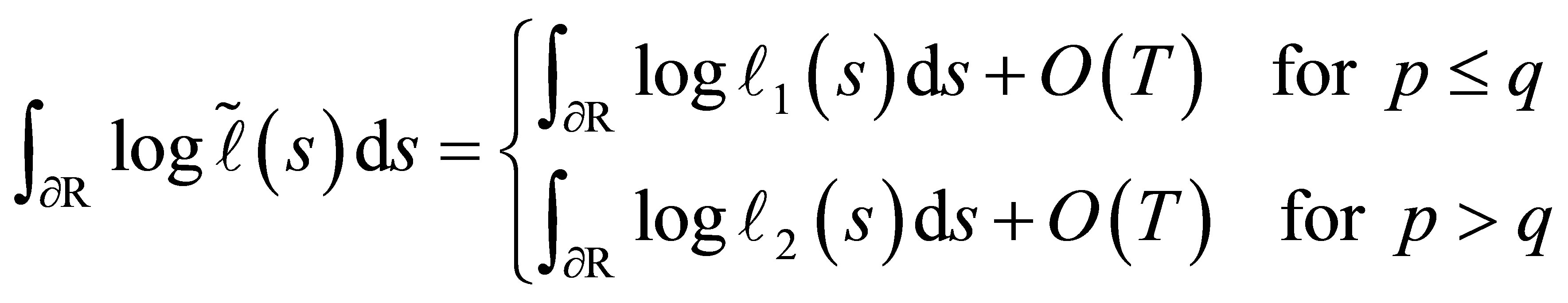
Finally, we estimate and. We show the computation for explicitly and note that the bound for follows analogously. We first suppose that has exactly zeros for. Then, there are at most subintervals, counting for multiplicities, in which is of constant sign. Thus,

(7)

It remains to estimate. To this end, we define

Then

so that if for, then.

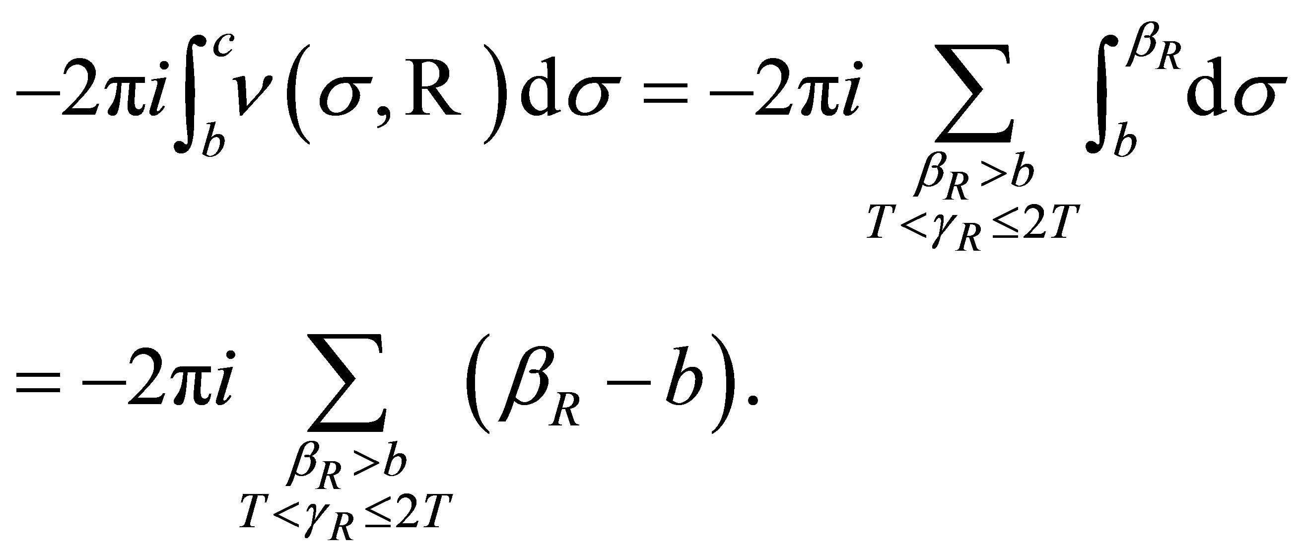
Now let and, and choose large enough so that. Then for, showing that no zeros or poles of are located in. Thus, both and are analytic in. Letting denote the number of zeros of in, we have

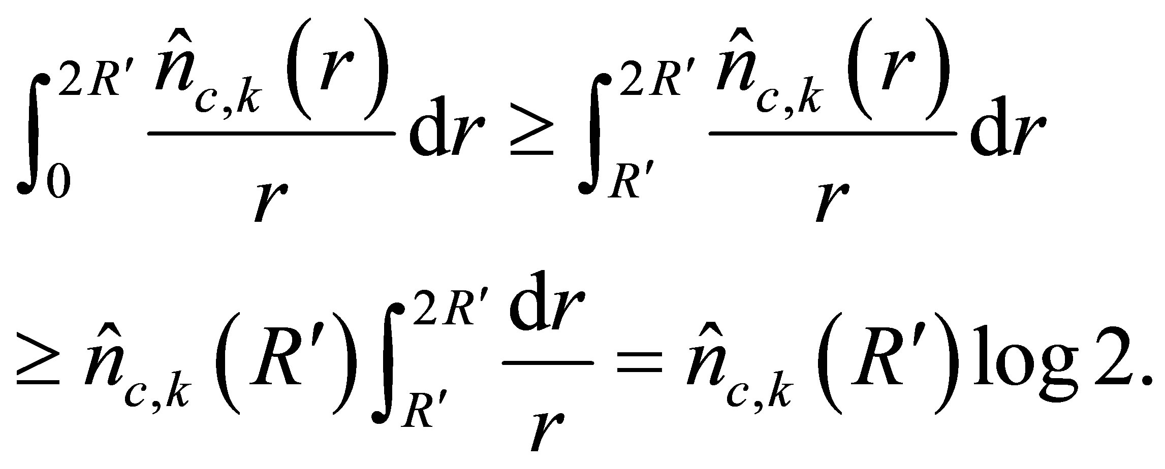
By Jensen’s formula

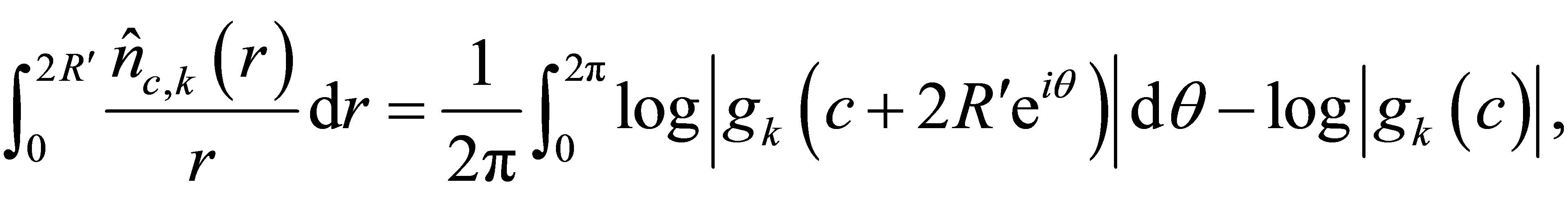
and so

(8)

(6)

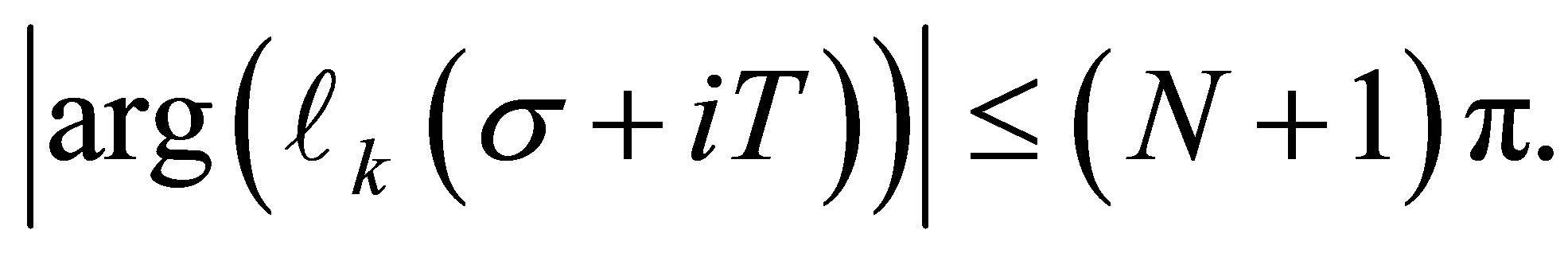
By (5), is bounded. Further, it is clear from a property of functions that we have

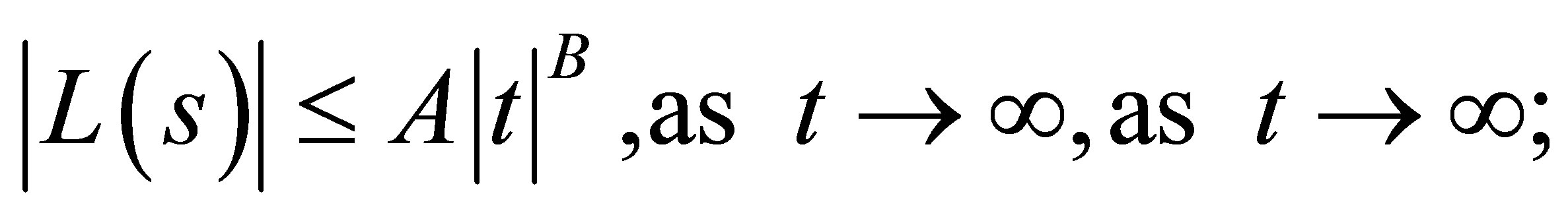
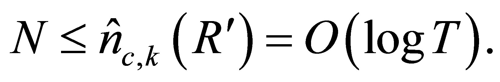
for some positive absolute numbers in any vertical strip of bounded width. The same estimate must hold for as well. Thus, the integral in (8) is, implying that . Since the interval, it follows that

With this bound, we integrate (7) to deduce that

As previously noted, we may bound in the same way. Thus, we attain the desired bounds for and. Consequently, the first part of the theorem is proved by using (4).

Proof of (II). As in the proof of the first part of the theorem, we conclude that there exists a real number for which the real parts of all -values satisfy; and also, there exist for each rational function such that no zeros of 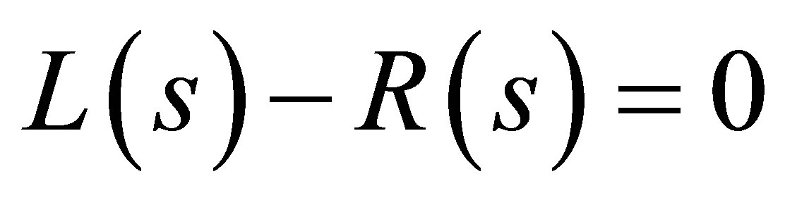lie in the quarter-plane. As before, we define the rectangl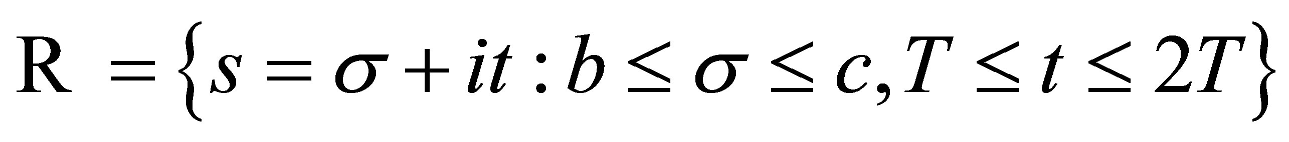e where are parameters satisfying .

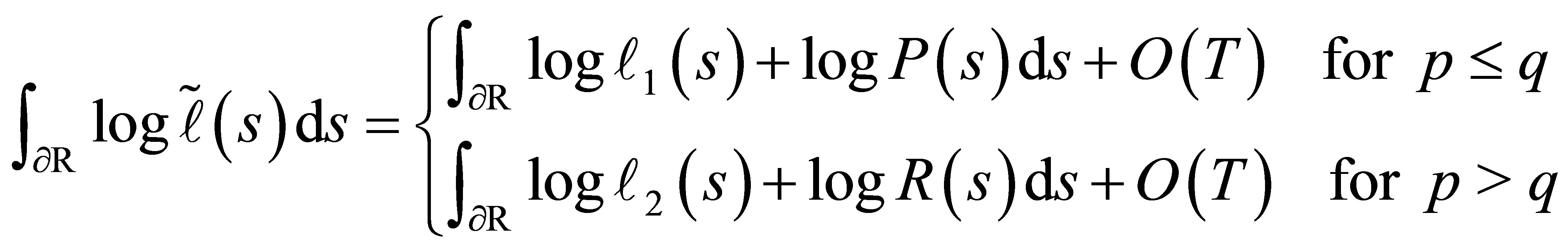
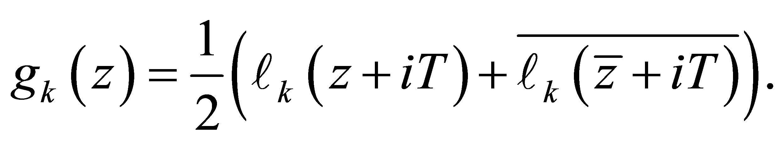
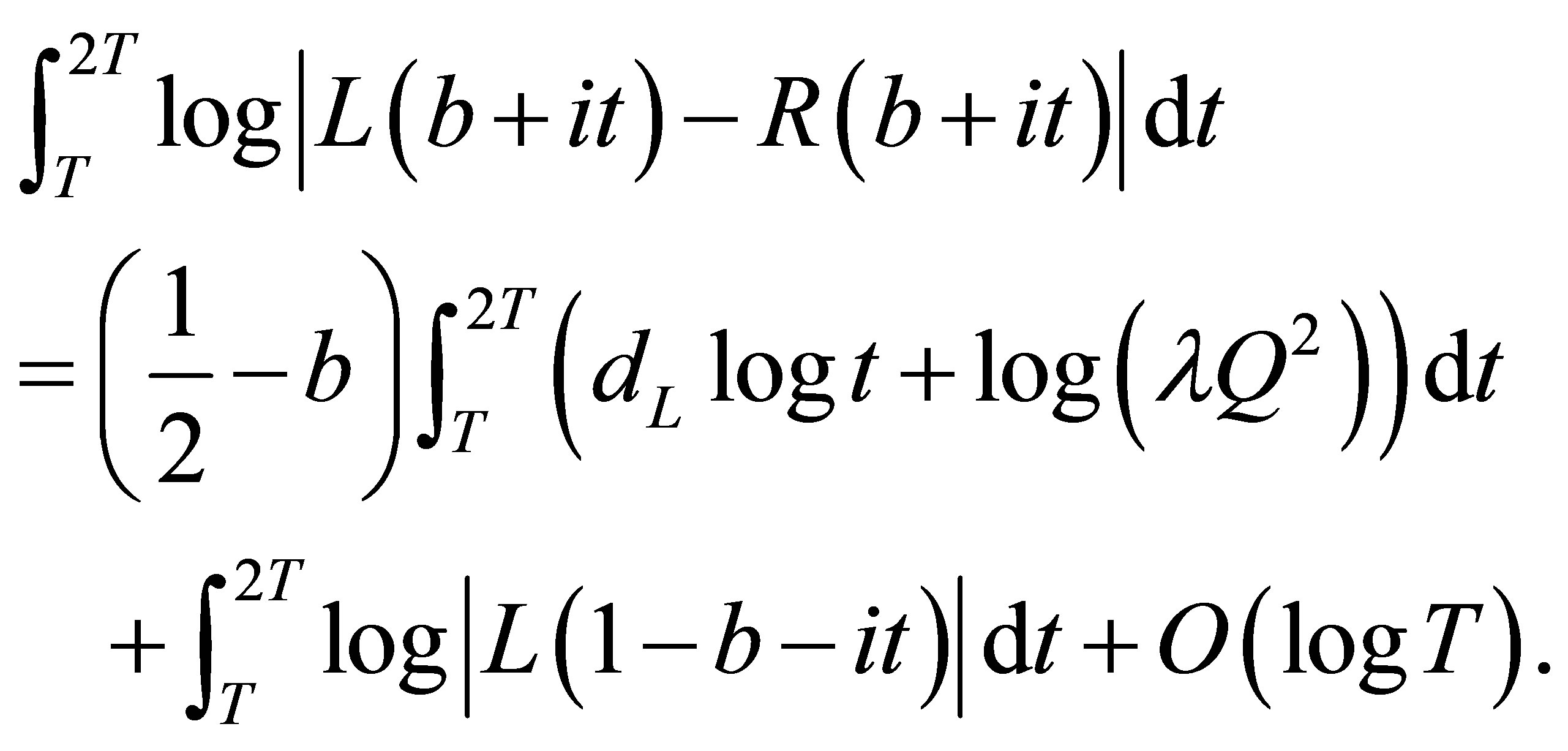
Proceeding as in the proof of the first part of the theorem, we see that

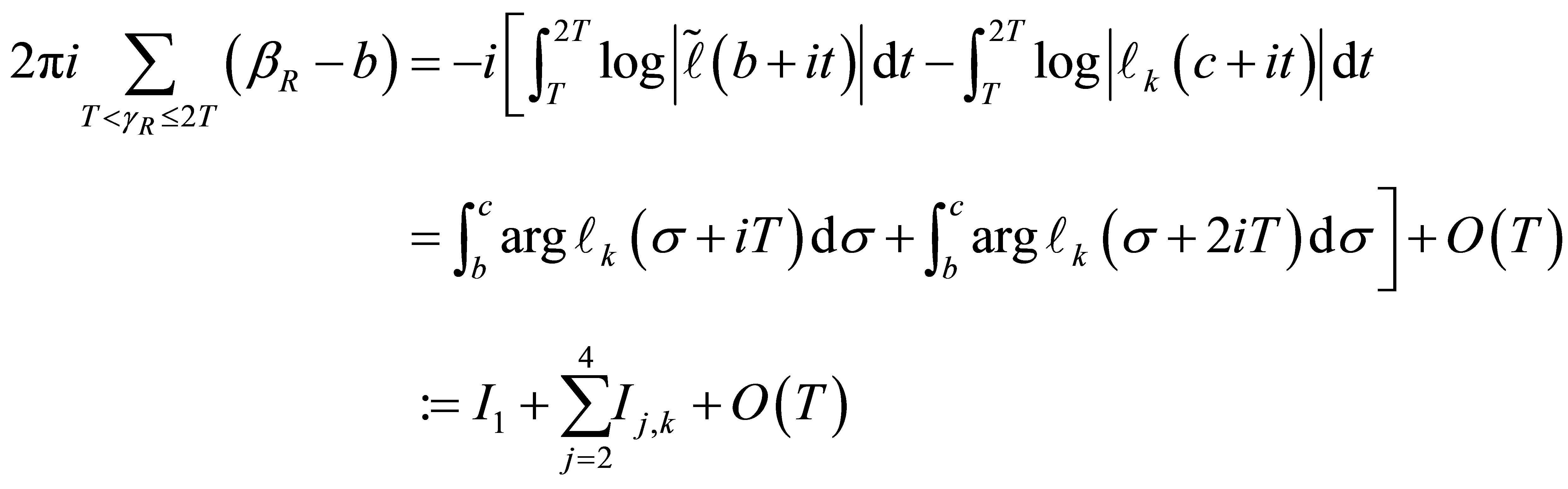
for where is defined as in (1). In the equation above, we note that we have chosen to compute separately. Indeed, this is the only estimate that we will need. For the integrals, and, the bounds given as in the proof of the first part of the theorem still hold. First, integral is unchanged. On the other hand, the integrals have changed by our choice of, but, as we have done as before, we still have the desired bound since the only requirement is that we consider in a vertical strip of fixed width, which we have in this case.

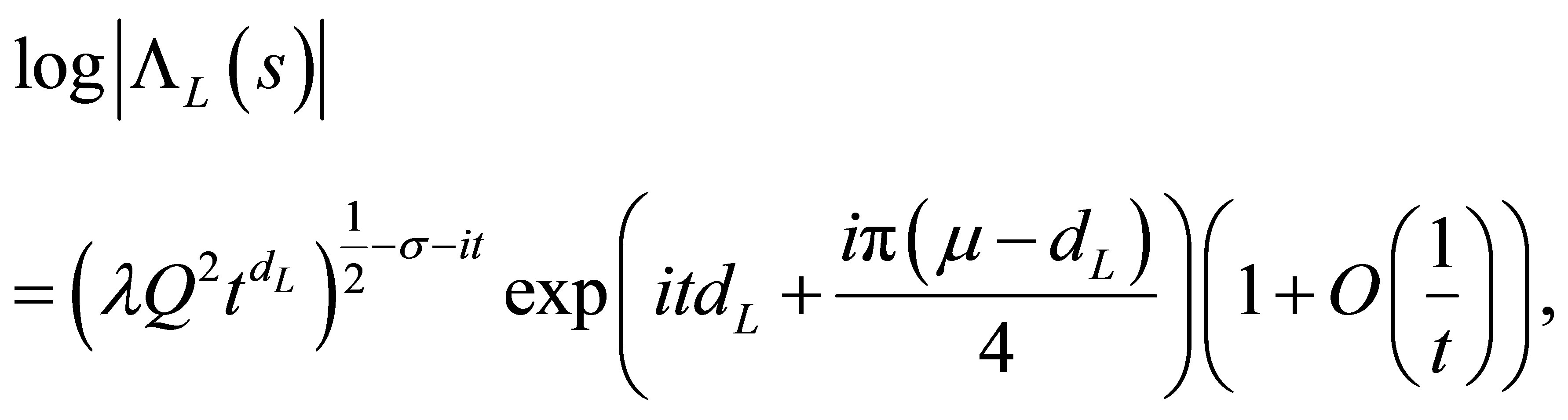
We now bound. Since, we have by the functional equation in the definition of function,

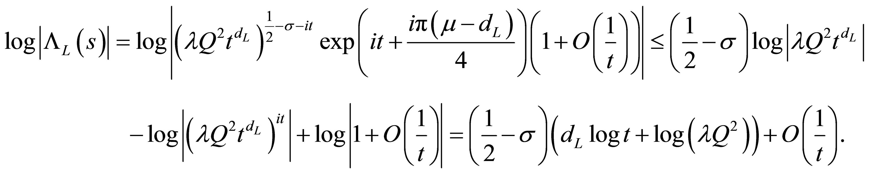
Taking logarithms, we get

(9)

Since, for, we have, uniformly in,

where are two constants. It follows, for as, that

We now consider the last term in (9). Since,

and noting, we have for any and

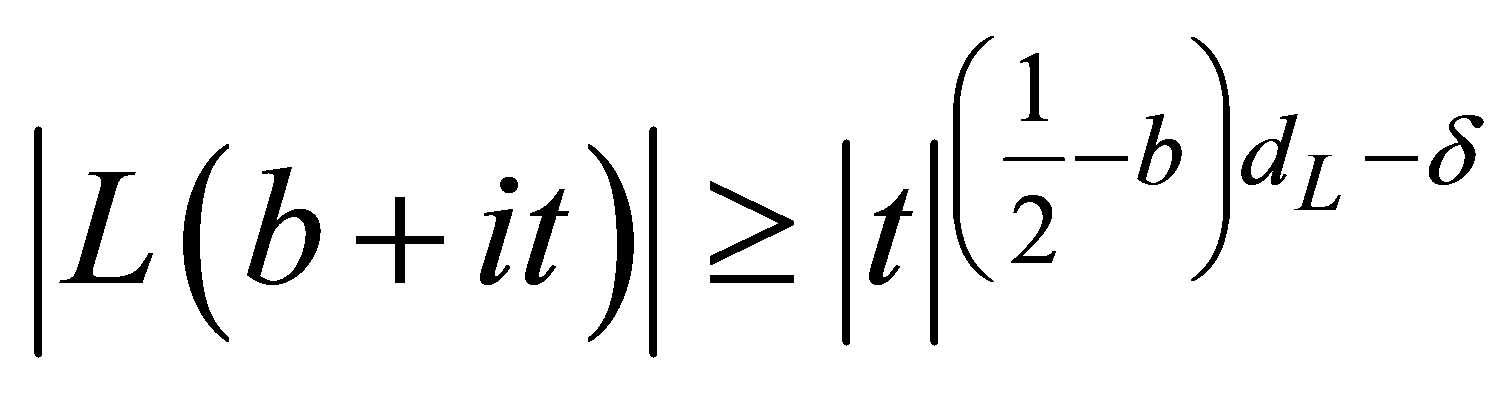
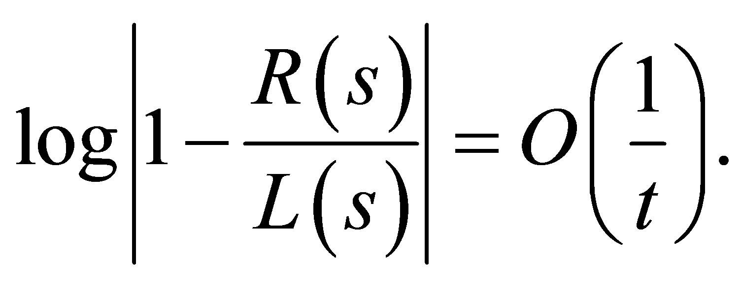
for sufficiently large. Then we see the quotient

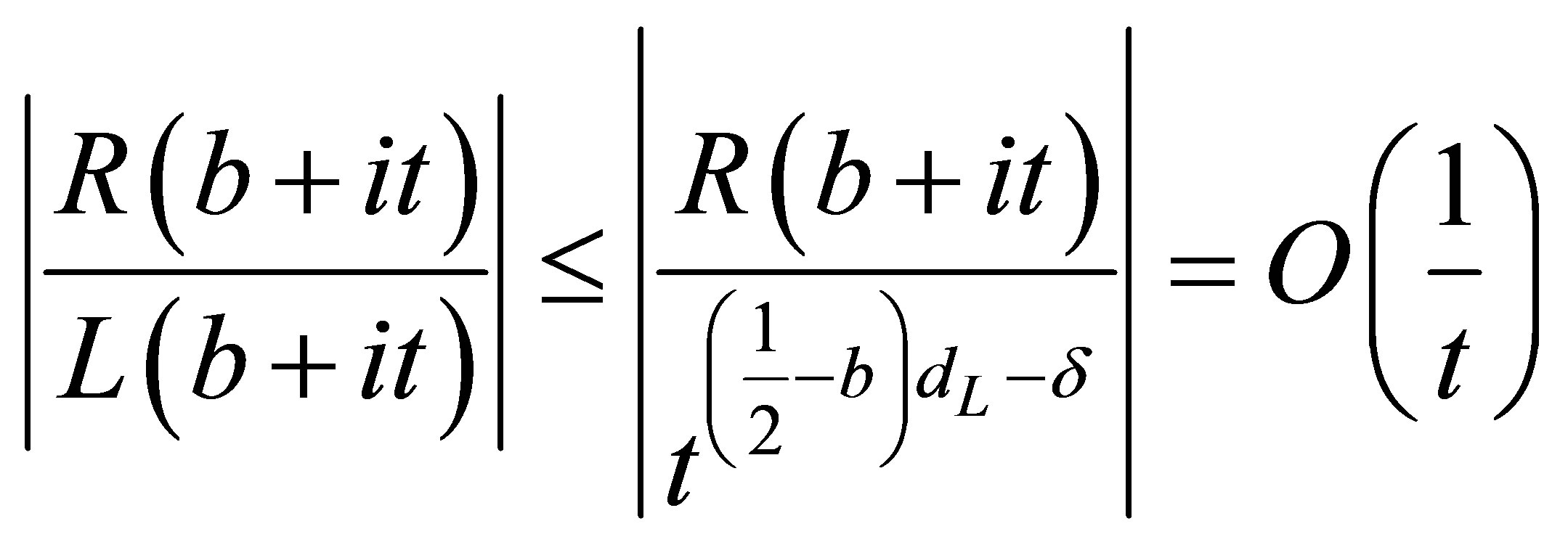
when is large enough so that

Therefore, we find that

Integrating in light of these estimates, we see

The first integral is, and the second integral is for sufficiently large and negative by the method used to derive (6). Hence,

With the estimates for the’s, we have proved the second part of the theorem.

REFERENCES

NOTES

^*Corresponding author.

REFERENCES

- J. Steuding, “Value Distribution of L-Functions,” Number 1877 in Lecture Notes in Mathematics, Springer, 2007.
- H. S. A. Potter, “The Mean Values of Certain Dirichlet Series I,” Proceedings London Mathematical Society, Vol. 46, No. 2, 1940, pp. 467-468. http://dx.doi.org/10.1112/plms/s2-46.1.467
- E. C. Titchmarsh, “The Theory of Functions,” 2nd Edition, Oxford, 1939.