World Journal of Mechanics
Vol. 1 No. 6 (2011) , Article ID: 16425 , 7 pages DOI:10.4236/wjm.2011.16038
A Finite Element Approximation of the Stokes Equations
1Laboratoire Génie Mécanique, Faculté des Sciences et Techniques, Fès, Maroc
2Mathématiques, Centre de Formation des Instituteurs Sefrou, Sefrou, Maroc
E-mail: elakkadabdeslam@yahoo.fr
Received September 1, 2011; revised October 15, 2011; accepted November 3, 2011
Keywords: Stokes Equations, Finite Element Method, Iterative Solvers, Adina System
ABSTRACT
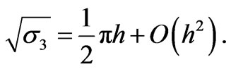
In this work, a numerical solution of the incompressible Stokes equations is proposed. The method suggested is based on an algorithm of discretization by the unstable of Q1 – P0 velocity/pressure finite element approximation. It is shown that the inf-sup stability constant is O(h) in two dimensions and O( ) in three dimensions. The basic tool in the analysis is the method of modified equations which is applied to finite difference representations of the underlying finite element equations. In order to evaluate the performance of the method, the numerical results are compared with some previously published works or with others coming from commercial code like Adina system.
1. Introduction
It is universally recognized that discretization schemes for Stokes and Navier-Stokes equations are subject to an inf-sup or div-stability condition [1]. The stability requirement is manifested in practical computations by the predominance of staggered grid finite volume discretizations, and the existence of unnatural velocity-pressure finite element combinations. These typically involve velocity bubble functions, or else have a macro-element definition of the velocity field.
A number of stabilization methods for inf-sup unstable approximations have been developed during the last three decades. These methods can be classified into two kinds. The first one is residual based stabilization, e.g. the absolutely stabilized method introduced by Douglas and Wang [2] and the Galerkin least square methods introduced by Franca and Hughes [3]. The other kind consists of pressure stabilized methods, and includes the global pressure jump stabilized method of Hughes and Franca [4].
In this paper the low order conforming finite element methods like  (trilinear/bilinear velocity with constant pressure) for incompressible flow problems are characterised.
The  finite element method is particularly controversial [1]. Despite being damned by theoreticians after the discovery of “weakly singular” modes [5,6],
  is widely used in practice. For the first time a clean analysis of the instability mechanism is presented.
Section 2 presents the model problem used in this paper. The discretization by finite elements is described in Section 3. Numerical experiments carried out within the framework of this publication and their comparisons with other results are shown in Section 4.
2. Governing Equations
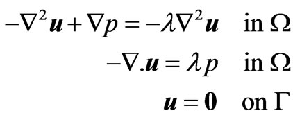
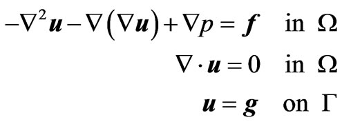
We consider the Stokes equations for the flow of an incompressible viscous fluid
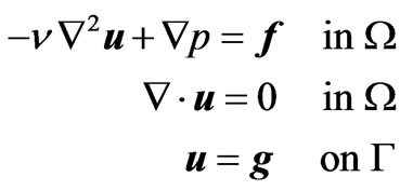 (1)
(1)
where  denotes the unit square with boundary
 .
.
v is a given constant called the kinematic viscosity, u is the fluid velocity, p is the pressure field and  is the gradient operator.
The geometry of the domain and boundary condition are shown in Figure 1.
3. Finite Element Approximation
In this section we introduce the finite element approximation of the Stokes equations in two dimensions, and we proceed to describe a means of estimating the relevant constant in the inf-sup condition. An alternative

Figure 1. Geometry of the domain and boundary condition for the velocity .
.
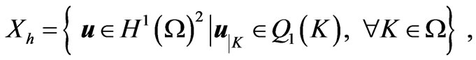
formulation is discussed at the end of this section. Assuming a grid of  square elements K, so that h = 1/n, an approximation based on the
 element uses function spaces
 (2)
(2)
 (3)
(3)
for velocity and pressure, respectively, where  is the space of bilinear functions and
  is the space of constant functions on K. The nodal positions of the
  element are illustrated in Figure 2. Denoting the velocity space satisfying homogeneous boundary conditions by
 , the finite element formulation is: find
  which interpolate the data
  at boundary nodes and
  such that
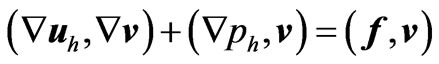 for all
  (4)
(4)
 for all
with standard interpolating bases for the spaces  and
and , this leads to the matrix system
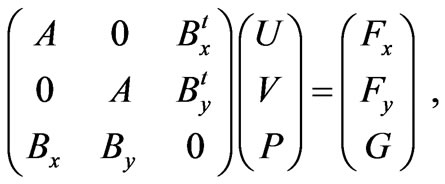 (5)
(5)
where U,  contain the nodal values of the x and y components of the approximation to
  at the internal vertices, and
  contains the element centroid values of the pressure approximation. The matrix A is of order
 , while both
  and
and  are of order
 , with
  and
and .
.
The satisfaction of the inf-sup condition is dependent on the eigenvalues  of
of
 (6)
(6)
where  is the
  mass matrix corresponding to the pressure space [7],
  represents
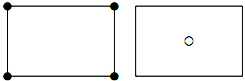
Figure 2.  element (● two velocity components; O pressure).
the discrete divergence operator and K is the vector Laplacian
 (7)
(7)
Since the discrete velocity field is specified everywhere on the boundary, the discrete Stokes operator has a two-dimensional null space spanned by the hydrostatic and chequerboard pressure modes [8]. Consequently, (6) has only  non-zero eigenvalues and we can order the eigenvalues so that
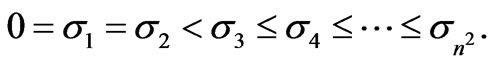 (8)
(8)
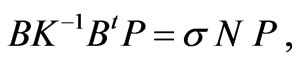
It may also be shown [7], that the nonzero eigenvalues of the “dual” problem
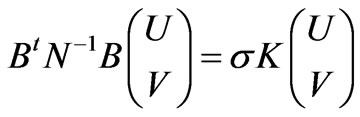 (9)
(9)
coincide with those of (6). We shall find it more convenient to work with the related eigenproblem
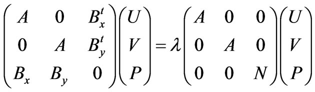 (10)
(10)
which reduces to (6) on elimination of U and V and to (9) on elimination of P. This system has an eigenvalue  of multiplicity equal to the dimension of the null space of the discrete divergence operator, that is
 , and the remaining
  eigenvalues are generated by the quadratic equation
  for
for :
:
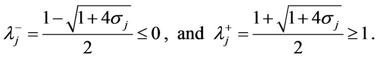 (11)
(11)
Applying the analysis of Brezzi and Fortin [1] or Malkus [7] the inf-sup stability of the system (4) (or, equivalently, (5)) is determined by the square root of the smallest non zero eigenvalue of (6) that is
 (12)
(12)
and we shall, accordingly, refer to  as the critical eigenvalue of (10) and denote it by
 . Experimental evidence reported in [2] suggests that
  as
as  indicating that
  is not div-stable in general. To investigate this issue further we write the constituent equations of (10) in finite difference form and then appeal to the method of modified equations. This will allow us to establish the precise behavior of
  for small values of h.
The x and y components of velocity at the grid point (lh, mh), l, m = 1, 2,···, n – 1 are labeled  respectively. The pressure is defined at element centroids
 , l, m = 0, 1 ···, n – 1 and is consequently labeled
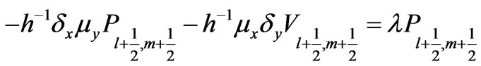
 . The system of Equations (10)
(each divided by ) may then be expressed as
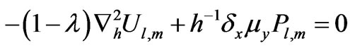
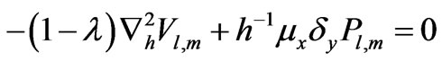 (13)
(13)
where
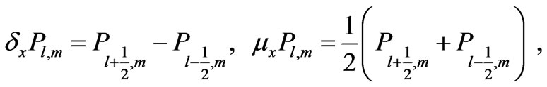 (14)
(14)
are the usual central difference and averaging operators, respectively, and  denotes the discrete Laplacian generated by bilinear elements
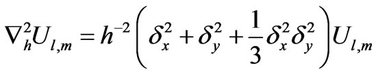 (15)
(15)
Figure 2 shows the  element and Figure 3 shows the pressure and the components of the velocity at the grid point.
Associated with (13) we have the boundary conditions  at nodes lying on the boundary
 . The system (13) is
 , (16)
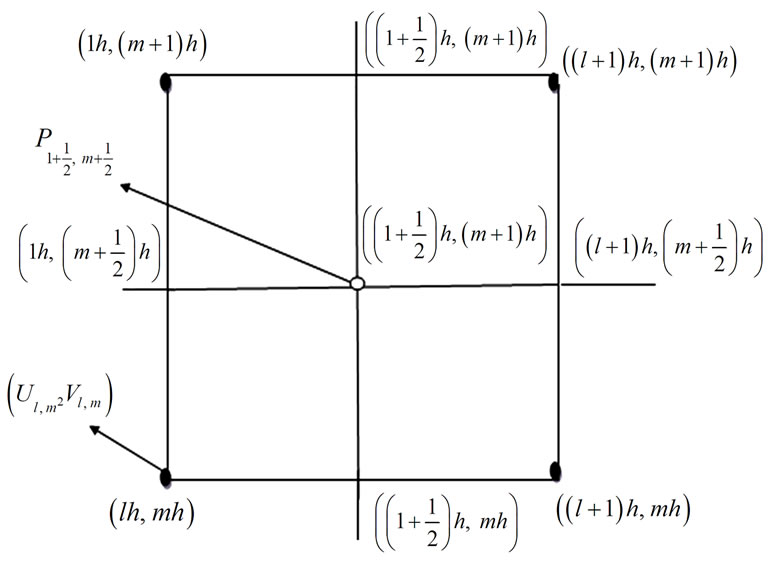
Figure 3. Pressure and the components of the velocity at the grid point.
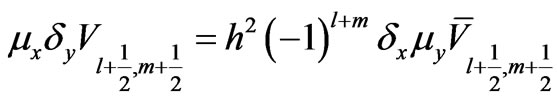
which has one eigenvalue  corresponding to the hydrostatic mode
 , p = constant, an eigenvalue
  of infinite multiplicity with corresponding eigenfunctions satisfying
  p = 0, and a pair of eigenvalues
 of infinite multiplicity corresponding to
and having irrotational eigenvectors .
.
In order to study the behavior of the critical eigenvalue , we assume that the corresponding eigenfunctions are highly oscillatory and have (smooth) envelopes
  defined by
 (17)
(17)
It then follows that
 (18)
(18)
So that
 (19)
(19)
Moreover,
 (20)
(20)
 (21)
(21)
 (22)
(22)
 (23)
(23)
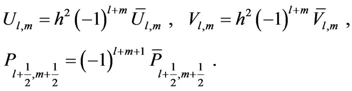
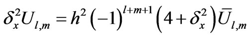
When these relations are used to change dependent variables in (13) from  to
to  we find that
 (24)
(24)
where , together with homogeneous Dirichlet boundary conditions on
  and
and . Denoting the Q1 basis function at node
  by
by , and supposing that
  has nodal values
 , thensince
 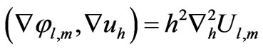 and
and
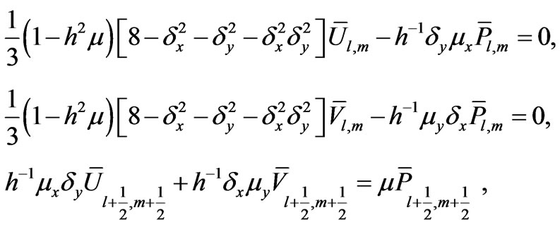
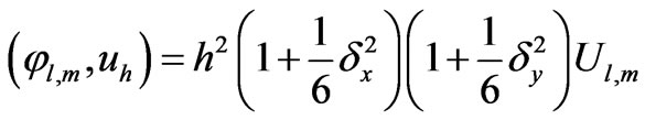 , it is easy to see that (24) is the Q1 – P0 discretization of the modified system
 (25)
(25)
In the limit  we obtain the reduced problem
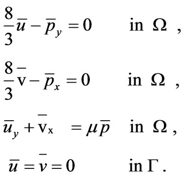 (26)
(26)
This implies that
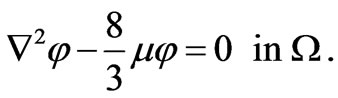 (27)
(27)
For each of the dependent variables . This, being a second order elliptic eigenvalue problem, requires only one boundary condition whereas the system (26) contains two. The Equations (25) therefore represent a singularly perturbed system [9] whose solutions will, in general, contain boundary layers. Bearing this in mind, we may identify the smallest non zero eigenvalue of (26) as
 (28)
(28)
associated with which there are two eigenfunctions, having outer expansions
 (29)
(29)
It is important to note that since  on
on ,it exhibits boundary layers of width O(h) along the vertical boundaries x = 0, 1. Similarly,
  has boundary layers of width O(h) along the horizontal boundaries y = 0, 1. We also note that, for this modified system, a “pressure gradient” in the y-direction induces a “flow” in the xdirection and vice-versa. We summarise in the form of a theorem.
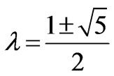
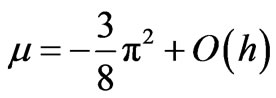
Theorem 1: The critical eigenvalue of (10) is given by 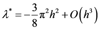 and the inf-sup constant for Q1 – P0 elements is given by
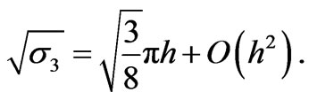 (30)
(30)
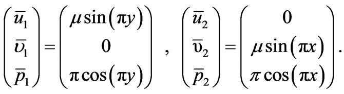
The eigenspace corresponding to  has dimension two and is spanned by mutually orthogonal eigenvectors given, approximately, by
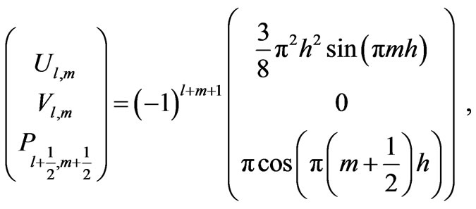 (31)
(31)
and
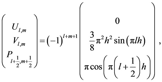 (32)
(32)
at internal nodes of the domain and  at boundary nodes. The amplitudes of the velocity and pressure contributions to these critical eigenvectors differ by a factor
 , which explains why, in computations, the instabilities manifest themselves most strongly in the pressure field. This will be explored further in the next section in connection with the model lid driven cavity problem.
An alternative Stokes formulation to (1) is the stress divergence form [1]:
 (33)
(33)
which after discretisation gives a matrix system which is slightly different to (5) above. If we discretise (33) using Q1 – P0 and follow the procedure described by (17) for changing variables, then it is easily shown that the resulting reduced problem is also of the form (26) except that the factor  is replaced by 4. In this case we have the result stated below.
Theorem 2: The inf-sup constant for Q1 – P0 approximation of (33) is given by
 (34)
(34)
The corresponding eigenspace has dimension two and is spanned by mutually orthogonal eigenvectors given, approximately, by (31) and (32).
4. Numerical Simulations
In this section, some numerical results of calculations with finite element method and ADINA system will be presented. Using our solver, we run the traditional test problem driven cavity flow [10-13].
We consider the critical eigenvalue of Theorem 1. The numerically computed eigenvalues  are presented in Table 1. The smallest eigenvalues are clearly tending to zero like O(h2).The largest eigenvalue is converging to an asymptotic limit of unity. Note also that for “unstable” eigenvalues: σj = O(h2) implies that
 (35)
(35)
Suggesting that  as
as 
Figures 4 and 5 show, respectively, the contours of pressure component of the first and the second unstable eigenvectors corresponding to , whereas Figures 6 and 7 show contours of pressure component of the unstable eigenvector corresponding to
  and those corresponding to
 .
.
The profiles of the u-velocity component along the vertical center line and the v-velocity component along the horizontal center line are shown in Figure 8. In this figure, we have the excellent agreement between the computed results and the results computed with ADINA system.
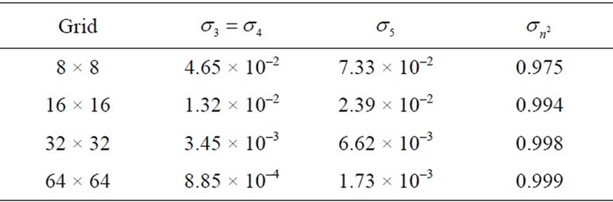
Table 1. Behavior of the eigenvalues  satisfying (6).
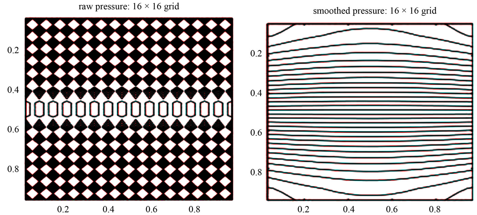
Figure 4. Contours of pressure component of the first unstable eigenvector corresponding to .
.
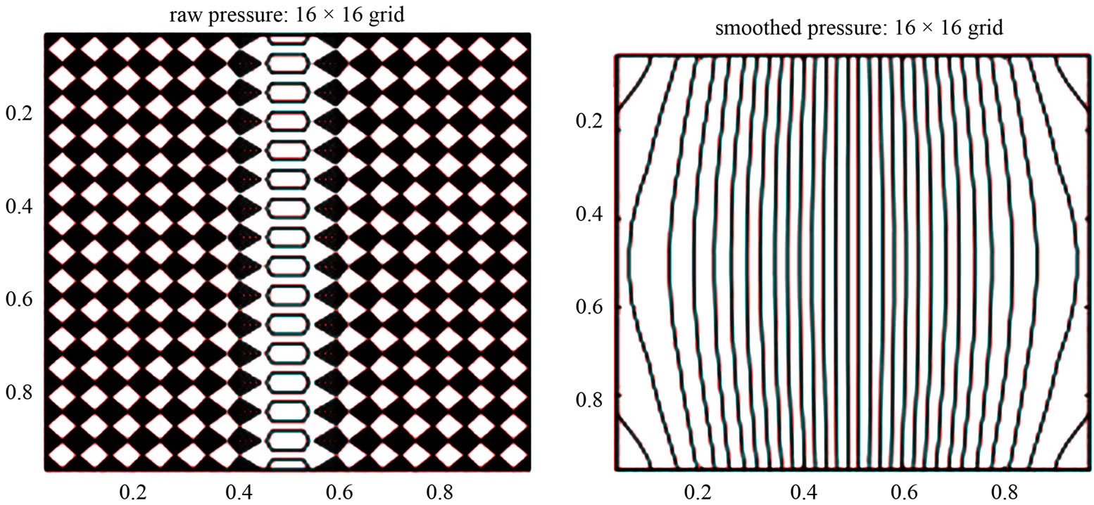
Figure 5. Contours of pressure component of the second unstable eigenvector corresponding to .
.
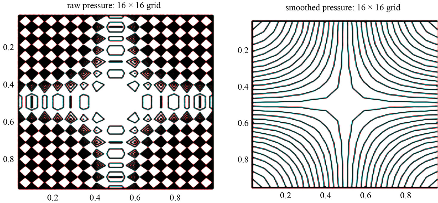
Figure 6. Contours of pressure component of the unstable eigenvector corresponding to .
.
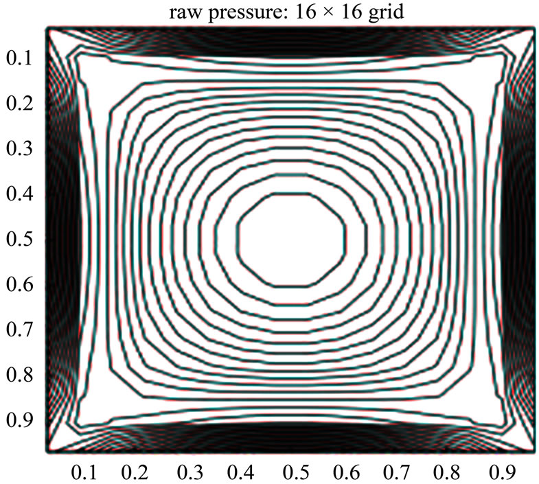
Figure 7. Contours of pressure component of the unstable eigenvector corresponding to .
.
5. Conclusions
We were interested in this work in the numerical solution for two dimensional differential equations model steady incompressible flow. It includes algorithms for discretization by finite element methods. For the test of drivencavity flow, the particles in the body of the fluid move in a circular trajectory.
Our results agree with Adina System.
Numerical results are presented to see the performance of the method, and seem to be interesting by comparing them with other recent results.
6. Acknowledgments
The authors would like to express their sincere thanks for the referee for his/her helpful suggestions.
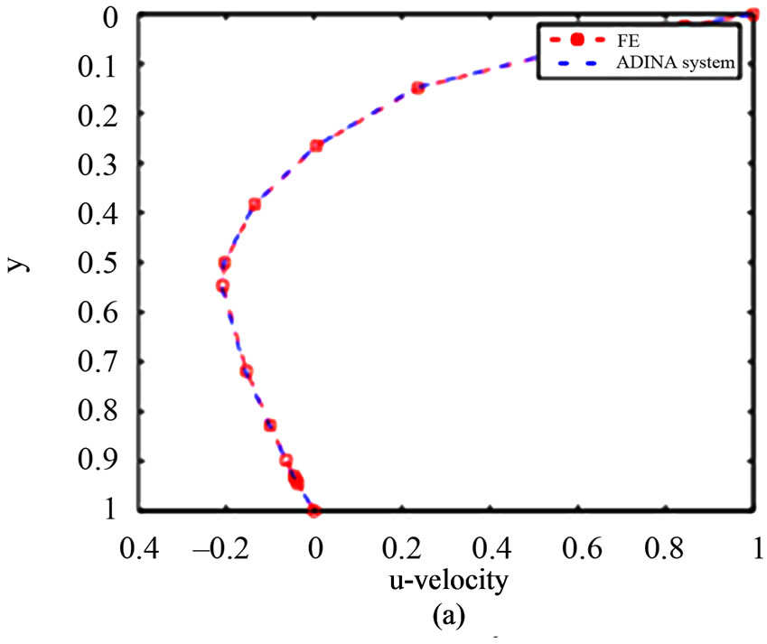
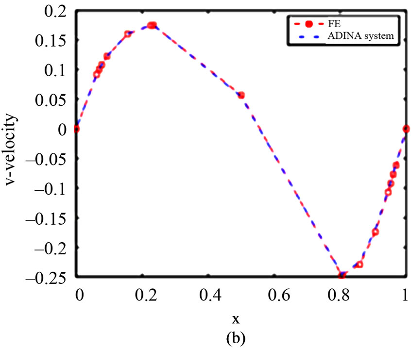
Figure 8. The velocity component u at vertical center line (a), and the velocity component v at horizontal center line (b) with a 129 × 129 grid.
REFERENCES
- F. Brezzi and M. Fortin, “Mixed and Hybrid Finite Element Methods,” Springer-Verlag, New York, 1991. doi:10.1007/978-1-4612-3172-1
- J. Douglas and J. Wang, “An Absolutely Stabilized Finite Element Method for the Stokes Problem,” Mathematics of Computation, Vol. 52, No. 186, 1989, pp. 495-508. doi:10.1090/S0025-5718-1989-0958871-X
- L. Franca and T. Hughes, “Convergence Analyses of Galerkin Least-Squares Methods for Symmetric Advectivediffusive Forms of the Stokes and Incompressible Navier-Stokes Equations,” Journal of Computer Methods in Applied Mechanics and Engineering, Vol. 105, No. 2, 1993, pp. 285-298. doi:10.1016/0045-7825(93)90126-I
- T. Hughes and L. Franca, “A New Finite Element Formulation for Computational Fluid Dynamics: VII. The Stokes Problem with Various Well-Posed Boundary Conditions: Symmetric Formulations That Converge for All Velocity/Pressure Spaces,” Journal of Computer Methods in Applied Mechanics and Engineering, Vol. 65, No. 1, 1987, pp. 85-96. doi:10.1016/0045-7825(87)90184-8
- J. Boland and R. Nicolaides, “On the Stability of Bilinear-Constant Velocity-Pressure Finite Elements,” Journal of Numerical Mathematics, Vol. 44, No. 2, 1984, pp. 219- 222. doi:10.1007/BF01410106
- J. Pitkaranta and R. Stenberg, “Error Bounds for the Approximation of the Stokes Problem Using Bilinear/Constant Elements on Irregular Quadrilateral Meshes,” In: J. Whiteman, Ed., The Mathematics of Finite Elements and Applications V, Academic Press, London, 1985, pp. 325- 334.
- D. Malkus, “Eigenproblems Associated with the Discrete LBB Condition for Incompressible Finite Elements,” International Journal of Engineering Science, Vol. 19, No. 10, 1981, pp. 1299-1310.
- R. Sani, P. Gresho, R. Lee and D. Grifiths, “The Cause and Cure (?) of the Spurious Pressures Generated by Certain Finite Element Method Solutions of the Incompressible Navier-Stokes Equations,” International Journal for Numerical Methods in Fluids, Vol. 1, No. 1, 1981, pp. 17-43. doi:10.1002/fld.1650010104
- J. Kevorkian and J. Cole, “Perturbation Methods in Applied Mathematics,” Springer-Verlag, New York, 1981.
- A. Elakkad, A. Elkhalfi and N. Guessous, “A Posteriori Error Estimation for Stokes Equations,” Journal of Advanced Research in Applied Mathematics, Vol. 2, No. 1, 2010, pp. 1-16. doi:10.5373/jaram.222.092109
- E. Erturk, T. C. Corke and C. Gokcol, “Numerical Solutions of 2-D Steady Incompressible Driven Cavity Flow at High Reynolds Numbers,” International Journal for Numerical Methods in Fluids, Vol. 48, No. 7, 2005, pp. 747-774. doi:10.1002/fld.953
- U. Ghia, K. Ghia and C. Shin, “High-Re Solution for Incompressible Viscous Flow Using the Navier-Stokes Equations and a Multigrid Method,” Journal of Computational Physics, Vol. 48, No. 3, 1982, pp. 387-395. doi:10.1016/0021-9991(82)90058-4
- S. Garcia, “The Lid-Driven Square Cavity Flow: From Stationary to Time Periodic and Chaotic,” Journal of Communications in Computational Physics, Vol. 2, 2007, pp. 900-932.