World Journal of Mechanics
Vol. 1 No. 5 (2011) , Article ID: 8164 , 10 pages DOI:10.4236/wjm.2011.15032
Influence of Inhomogeneity and Initial Stress on the Transient Magneto-Thermo-Visco-Elastic Stress Waves in an Anisotropic Solid
Faculty of Computers and Informatics, Suez Canal University, Ismailia, Egypt
E-mail: mafahmy2001@yahoo.com
Received July 14, 2011; revised August 16, 2011; accepted September 2, 2011
Keywords: Magneto-Thermoviscoelastic Stresses, Initial Stress, Inhomogeneity, Anisotropic, Dual Reciprocity Boundary Element Method
ABSTRACT
The object of the present paper is to study the transient magneto-thermo-visco-elastic stresses in a non-homogeneous anisotropic solid under initial stress. The system of fundamental equations is solved by means of a dual reciprocity boundary element method (DRBEM). In the case of plane deformation, a numerical scheme for the implementation of the method is presented and the numerical computations are presented graphically to show the effects of initial stress and inhomogeneity on the displacement components and thermal stress components.
1. Introduction
An increasing attention is being devoted to the interaction between magnetic field and strain field in an initially stressed anisotropic viscoelastic solid due to its many applications in modern aeronautics, astronautics, earthquake engineering, soil dynamics, nuclear reactors and high-energy particle accelerators. In recent years, an important number of engineering and mathematical papers devoted to the numerical solution have studied the overall behavior of such materials. El-Naggar, et al. [1,2] proposed explicit finite difference scheme to obtain thermal stresses in a non-homogeneous media. The boundary element method is well known for its accuracy and efficiency in stress analysis (see, for example, Brebbia and Nardini [3], Wrobel and Brebbia [4], Partridge, et al. [5], Divo and Kassab [6], Gaul, et al. [7], Matsumoto, et al. [8], Fahmy [9-11], Davi and Milazzo [12]).
The idea of the present paper is to study the transient magneto-thermo-visco-elastic stresses in a non-homogeneous anisotropic initially stressed solid. The formulation is tested through its application to the problem of a solid placed in a constant primary magnetic field acting in the direction of the z-axis. The governing equations are solved by means of a dual reciprocity boundary element method (DRBEM) and then numerical calculations are made for the temperature, displacement components and thermal stress components. The validity of DRBEM is examined by considering a magneto-thermo-viscoelastic solid occupies a rectangular region and good agreement is obtained with existent results. The results indicate that the effects of initial stress and inhomogeneity are very pronounced.
2. Formulation of the Problem
Here, we present the basic equations of the theory of magneto-thermoviscoelasticity, which will be used for the solution of the problem described above. With reference to a Cartesian frame denoted by 0xyz, consider an initially stressed anisotropic solid is placed in a constant primary magnetic field H0, acting in the direction of the z-axis. Here we address the generalized two-dimensional deformation problem in xy-plane only, therefore all the variables are constant along the z-axis. In the 0xy plane, the solid occupies the region
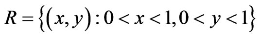 which is bounded by a simple closed curve C.
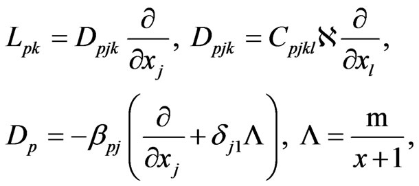
In non-dimensional form the governing equations of magneto-thermo-viscoelasticity for an anisotropic solid can be written as follows (see Fahmy and El-Shahat [13])
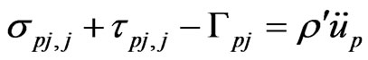 (1)
(1)
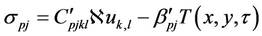 (2)
(2)
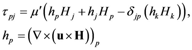 (3)
(3)
 (4)
(4)
 (5)
(5)
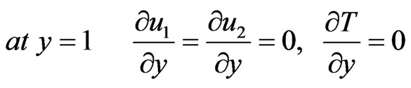
The initial and boundary conditions for the current problem are assumed to be written as
 (6)
(6)
 (7)
(7)
 (8)
(8)
 (9)
(9)
 (10)
(10)
 (11)
(11)
where  and
and  are the same expressions
  and
and  respectively,
  is the mechanical stress tensor,
  Maxwell’s electromagnetic stress tensor,
  is the displacement, T is the temperature,
  is the initial stress in the solid,
  and
and  are respectively, the constant elastic moduli and stress-temperature coefficients of the anisotropic medium,
  is the viscoelastic material constant,
  is the magnetic permeability,
  is the perturbed magnetic field,
  are the thermal conductivity coefficients satisfying the symmetry relation
  and the strict inequality
  holds at all points in the medium,
  is the density,
  is the specific heat capacity of the solid and
  is the dimensionless time,
  is the heat source density and
  is the Euclidean distance between the field point
  and the load point
 . Also,
  ,
,  and
and  are suitably prescribed functions of
 ,
,  is suitably prescribed function of
 ,
,  and
and  are nonintersecting curves such that
 ,
,  and
and  are non-intersecting curves such that
  and
and  are the tractions defined by
 .
.
A superposed dot denotes differentiation with respect to the time and a comma followed by a subscript denotes partial differentiation with respect to the corresponding coordinates.
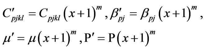
We focus our attention to the case of inhomogeneity along x-axis, so we characterize the elastic constants , magnetic permeability
 , initial stress
 , thermal conductivity coefficients
  and density
  of non-homogeneous material by
 (12)
(12)
 (13)
(13)
where ,
,  ,
,  ,
,  and
and  are constants (the values of
 ,
,  ,
,  ,
,  and
and 
 in homogeneous matter) and m is a rational numbers.
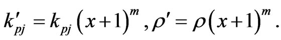
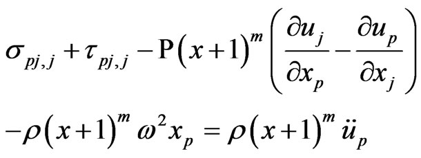
In terms of the definitions (12) and (13), Equations (1) and (5) can be written as follows
 (14)
(14)
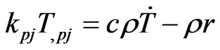 (15)
(15)
With the heat flux vector  given by Fourier’s law
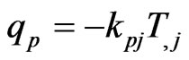 (16)
(16)
where  and
and  are taken to be constant in
 .
.
It is usually difficult to find out the analytical solutions of such state equations except for some special cases.
3. Numerical Implementation
The main objective of the numerical implementation is to describe the implementation of the DRBEM formulation for the solution of the equations (14) and (15). A more extensive historical review and applications of dual reciprocity boundary element method may be found in Brebbia, et al. [14], Partridge and Wrobel [15], Nardini and Brebbia [16], Albuquerque, et al. [17].
3.1. Temperature Field
Weighting (15) with a test function  yields
 (17)
(17)
Applying Gauss’s theorem, integration by parts, Green’s second identity and sifting property of the Dirac distribution, we obtain the representation formula
 (18)
(18)
According to the DRBEM, the surface of the solid has to be discretized into boundary elements. In order to make the implementation easy to compute, we use  collocation points on the boundary
  and another
  in the interior of
  so that the total number of interpolation points is
 .
.
According to Cho, et al. [18], a function of the form
where  is a continuous function in the
  -plane and
  is a polynomial of degree
  is called a radial basis function (RBF). The importance of splines is that they can provide interpolatory approximations to
  for very general sets of interpolation points
  in the xyplane.
In the  -plane a spline is of the form
 (19)
(19)
where  is the Euclidean distance between the field point
  and the load point
 . and
. and  is a polynomial of degree
 . For
. For  these are the thin plate splines (TPS)
 and
and 
Thus, the particular solution of the temperature can be approximated as
 (20)
(20)
where
and
Consequently, the dual reciprocity representation formula can be written as follows
 (21)
(21)
in which all domain integrals have been transformed to the boundary.
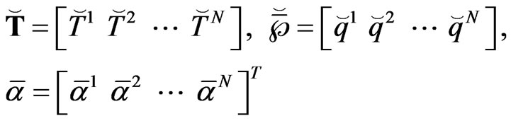
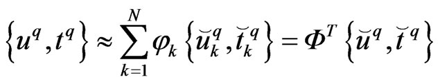
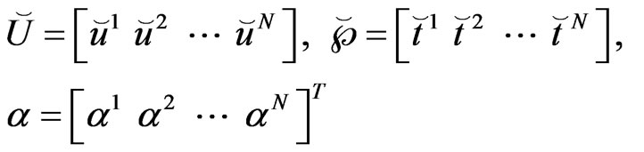
The field variables  and
and  are then approximated by means of shape functions
  and nodal values
  and
and  as follows
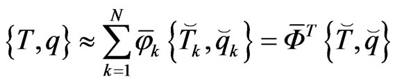 (22)
(22)
where ,
,  and
and  are matrices We can also approximate the particular solutions
  and
and  on the boundary as the unknown field variables by means of nodal values
  and
and  as follows
 (23)
(23)
where  and
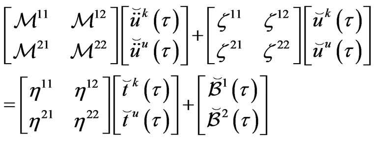
and  are matrices Using (22) and (23) and applying the point collocation procedure to (21), we have the following system of equations
 (24)
(24)
Let
 (25)
(25)
Using (25) into (24) we have
 (26)
(26)
where the matrices  and
and  contain the particular solutions.
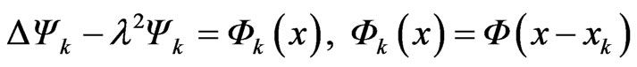
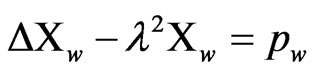
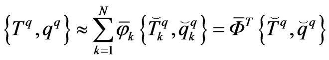
The generalized source term in (18) is approximated with a series of given source source terms  and unknown coefficients
  as follows
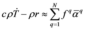 (27)
(27)
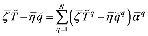
Then, by applying a point collocation procedure to equation (27) we obtain
 (28)
(28)
which can be substituted into (27) producing
 (29)
(29)
where
 (30)
(30)
In order to solve the system (29), the nodal vectors are subdivided into known and unknown parts denoted by the superscripts  and
and 
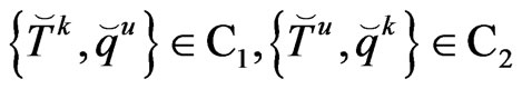 (31)
(31)
The following matrix equation is obtained from (29):
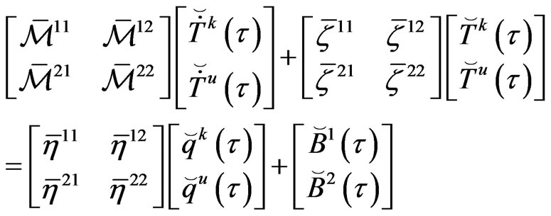 (32)
(32)
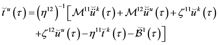
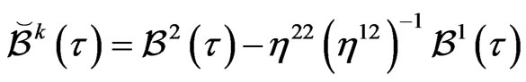
The unknown fluxes  are obtained from the first row of matrix equation (32) are expressed as follows
 (33)
(33)
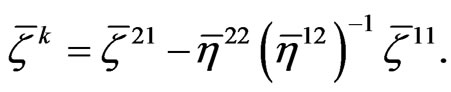
Making use of (33) we can write the second row of matrix equation (32) as follows
 (34)
(34)
where

At a time step , equation (34) can be written in the following form
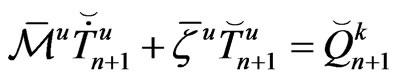 (35)
(35)
where

We take the finite difference grids with  as the time step, and use the subscripts
  to denote the
  discrete time. A mesh is defined by
 ,
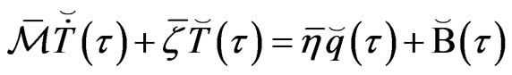
,  being the time step Using finite difference, we can approximate the temperature as follows
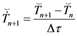 (36)
(36)
Hence, we can write
 (37)
(37)
where
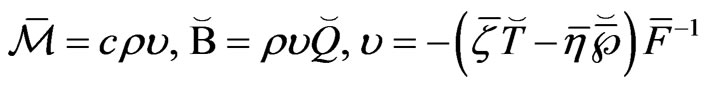
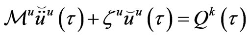
Thus, with  determined, the remaining task is to solve (14) subject to (6), (7) and (8).
3.2. Displacement Field
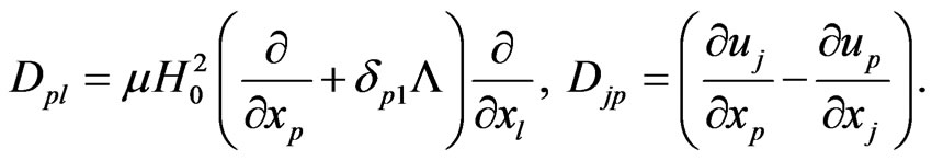
Making use of (2)-(4), (12) and (13), we can write (14) as follows
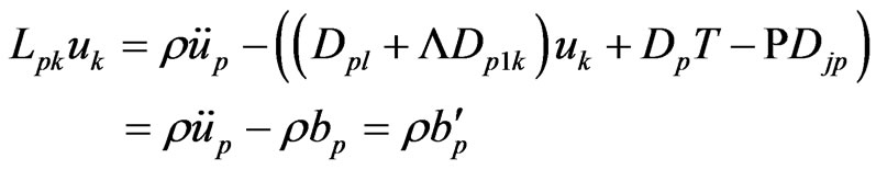 (38)
(38)
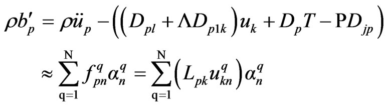
where
When the temperature field is known, the displacement field is obtained by solving (38), where the inertia term , the magnetic term
 , the viscosity term
 , the temperature gradient
  and the initial stress term
  are treated as the body forces.
On the basis of the method of weighted residuals, the differential equation (38) can be transformed to the integral equation in the following form
 (39)
(39)
where  is a weighting function and
  is the approximate solution.
Integration by parts twice using the divergence theorem of Gauss as in Fahmy [11] yields
 (40)
(40)
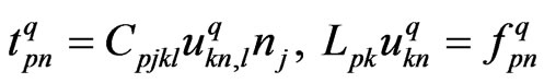
where the traction vectors on the boundary are
 (41)
(41)
Using the symmetric elasticity tensor 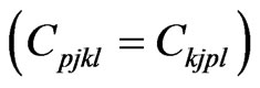 Therefore, it follows that
 (42)
(42)
 (43)
(43)
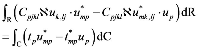
Using equations (41), (42) and (43), the equation (40) can now be rewritten in the form
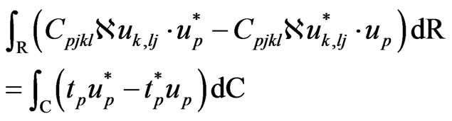 (44)
(44)
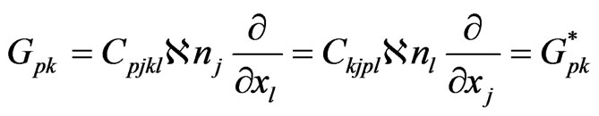
We define the fundamental solution  by the relation
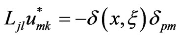 . (45)
If we replace the weighting functions  in (44) by
 , then we have
 (46)
(46)
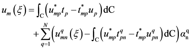
From (38), (45) and (46), the representation formula may be written as
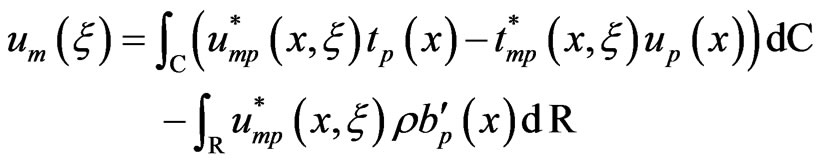 (47)
(47)
Let
 (48)
(48)
Using the TPS as in Cho, et al. [18], we can write the particular solution of the displacement as follows
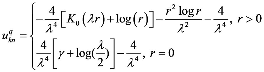 (49)
(49)
where  is the Bessel function of the third kind of order zero and
 , which is known as Euler’s constant.
Hence, the traction particular solution  and source function
  can be obtained by evaluating
 (50)
(50)
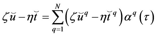
On the basis of these considerations, the integral domain can be approximated as
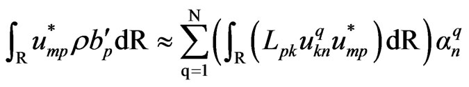 (51)
(51)
The use of (51) together with the dual reciprocity
 (52)
(52)
Gives rise to
 (53)
(53)
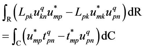
From (45), one may derive
 (54)
(54)
Making use of (47), (53) and (54) we can write the dual reciprocity representation formula as follows
 (55)
(55)
The representation formula (55) is only valid if  lies inside the domain
 . To obtain an expression that contains only boundary variables, the load point
  has to be moved to the boundary. Therefore, the boundary is deformed by a small circular region with radius
  around the load point
 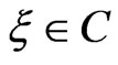 as shown in Figure 1.
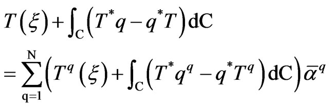
According to references [11], [19] and [20], the dual reciprocity boundary integral equation can be expressed as
 (56)
(56)
where ∮ is the Cauchy principal value symbol.
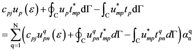
The unknown field variables and the particular solutions are respectively approximated by means of nodal values  and shape functions
 (57)
(57)
 (58)
(58)
where  and
and  are matrices.
On the basis of these approximations, and using the point collocation procedure, the dual reciprocity boundary integral equation (56) results to the following system of equations
 (59)
(59)
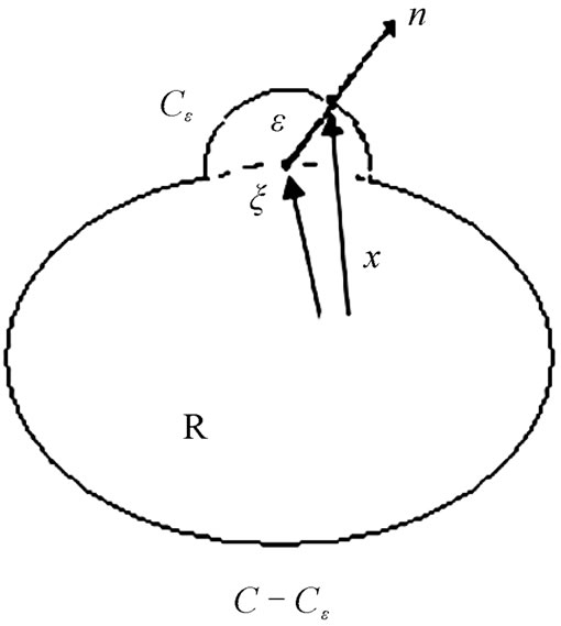
Figure 1. Geometry of the deformed boundary.
By letting
 (60)
(60)
We can write (59) as follows
 (61)
(61)
The coefficient vector  can be calculated from (48) using the point collocation procedure, which yields
 (62)
(62)
Thus, (61) yields the system
 (63)
(63)
where
 (64)
(64)
By subdividing the nodal vectors into known and unknown parts as follows
 (65)
(65)
where the superscripts  and
and  denote, respectively, the known and unknown parts Hence we can write the system (63) in the following form
 (66)
(66)
The unknown fluxes 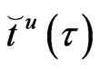 can be obtained from the first row of (66) as follows
 (67)
(67)
With the aid of (67) into the second row of (66) we obtain
 (68)
(68)
where

We can write (68) at time step 
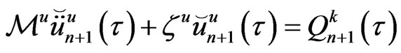 (69)
(69)
where

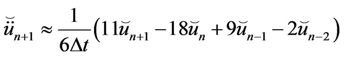
Now, we consider an implicit backward finite difference scheme for solving the system of ordinary differential equation (69), the so-called Houbolt’s algorithm is applied to reduce (69) to an algebraic system. To do this, the velocities  and accelerations
  at time step
  are approximated as follows
 (70)
(70)
 (71)
(71)
Substituting (94) and (95) into (93) we have
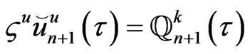 (72)
(72)
where
We apply successive over-relaxation (SOR) as described in Golub and Van Loan [21] to solve the system (96). For every time step  the values of
  are established. Once these values have been obtained, the unknown
  and
and  can be obtained from (70) and (71), respectively. For the case in which
 , the procedure described in Bathe [22] is used together with the initial conditions to derive
  and
and . Lastly, we compute the traction vector
  using (67).
4. Numerical Results and Discussion
The present work should be applicable to any magneto-thermo-viscoelastic deformation problem. The application is for purpose of illustration; we do not intend to validate the results in a quantitative way because we have no experimental data at hand; this may be justified because our objective is to introduce a viable numerical technique for studying a model rather than to study any physical behaviors of it (see, for example, Ahmed [23], Kanaun [24] and Monsia [25]). Such a technique was discussed in Abd-Alla et al. [26-28] who solved the special case from this study in the absence of viscosity and inertia. To achieve better efficiency than the technique described in Abd-Alla, et al. [26-28], we use thin plate splines into a code, which is proposed in the current study. We extend the study of Abd-Alla, et al. [26-28], to include the viscosity interactions and the inertia term. Thus, it is perhaps not surprising that the numerical values obtained here are in very good agreement with those obtained by Abd-Alla et al. [26-28].
The example considered by Sladek, et al. [29] may be considered as a special case of the current general problem in the context of the uncoupled thermoelasticity theory. Also, there are alot of practical applications may be deduced as special cases from this general study and may be implemented in commercial finite element method (FEM) software packages FlexPDE 6.
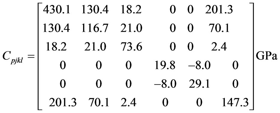
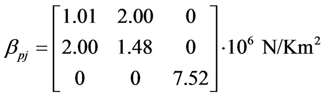
In the special case under consideration, the results of the displacement  are plotted in Figure 8 to show the validity of the proposed method. These results obtained with the DRBEM have been compared graphically with those obtained using the Meshless Local Petrov-Galerkin (MLPG) method of Sladek, et al. [29] and also the results obtained from the FlexPDE 6 are shown graphically in the same figures to confirm the validity of the proposed method. It can be seen from this figure that the DRBEM results are in excellent agreement with the results obtained by MLPG and finite element methods, thus confirming the accuracy of the DRBEM.With a view to illustrate the numerical implementation presented earlier, we consider a monoclinic graphite-epoxy as an anisotropic magneto-thermo-visco-elastic solid with the following physical constants:
Elasticity tensor
Mechanical temperature coefficient
Tensor of thermal conductivity
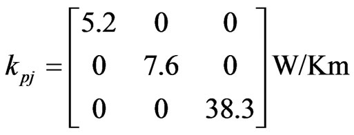
Mass density 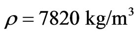 and heat capacity
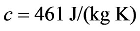 ,
, 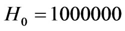 Oersted,
  Gauss/Oersted,
  ,
,  ,
, . The boundary
  is
is , the boundary
  is
is , the boundary
  is
is , while
  is
is . The numerical values of the temperature and displacement are obtained by discretizing the boundary into 120 elements
  and choosing 60 well spaced out collocation points
  in the interior of the solution domain.
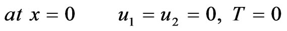
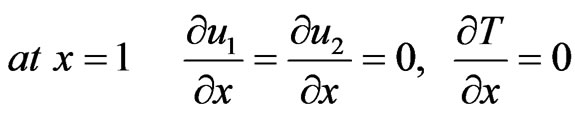
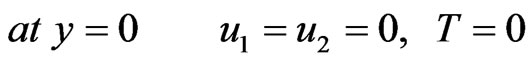
The initial and boundary conditions considered in the calculations are

In order to evaluate the influence of the inhomogeneity on the displacements and thermal stresses in an anisotropic viscoelastic solid under initial stress, the inhomogeneity parameter is taken to be  and for the homogeneous solid, we assume that
 .
.
A comparison of the results is presented graphically for the following different cases: the solid line denoted by “A” represents the solution for homogeneous solid in the absence of initial stress , the dashed line denoted by “C” represents the solution for non-homogeneous solid in the absence of initial stress, the dotted line denoted by “B” represents the solution for homogeneous solid in the presence of initial stress
 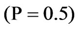 and the dashed-dotted line denoted by “D” represents the solution for non-homogeneous solid in the presence of initial stress.
Figure 2 shows the variation of the temperature T along  -axis at various values of the time
 . It is noticed that the temperature increases with the increase of
  and
and .
.
Figures 3-7 show the influence of the initial stress and inhomogeneity of the material constants on the displacements  and
and  and thermal stresses
 ,
,  and
and . Also, they show the difference among the four cases “A”, “C”, “B” and “D”.
Figure 3 shows that the displacement  increases and then decreases with the increase of
 . It is noticed that the maximum value happens in the homogeneous solid in the presence of initial stress.
Figure 4 shows that the displacement  decreases and then increases for all cases. It is clear from this figure that the homogeneous and non-homogeneous curves
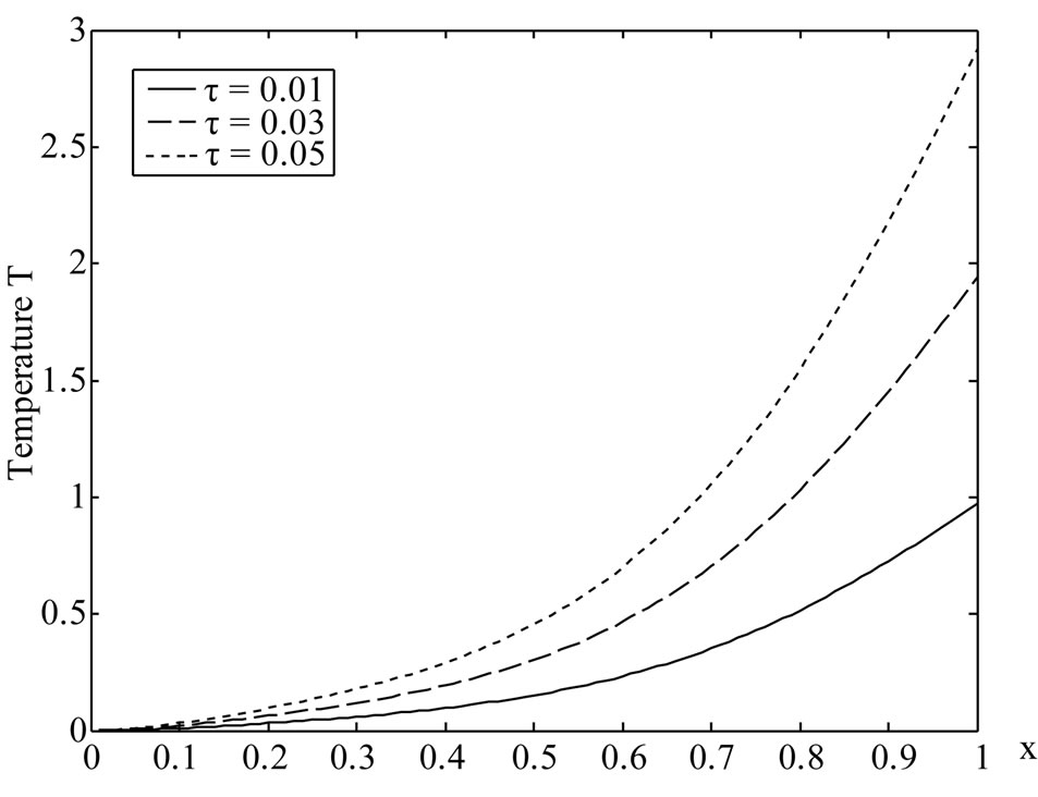
Figure 2. Variation of the temperature T with x coordinate (y = 1).
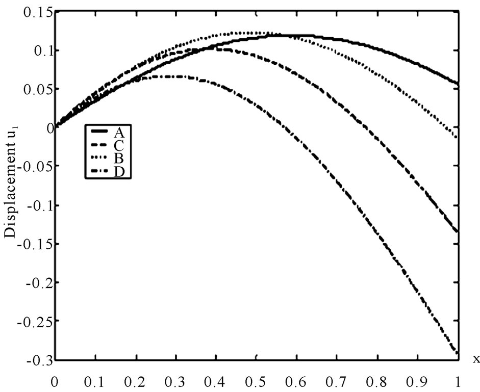
Figure 3. Variation of the displacement u1 with x coordinate.
Figure 4. Variation of the displacement u2 with x coordinate.
diverge in the presence of initial stress. We can see also from this figure that the negative maximum value happens in the non-homogeneous solid in the presence of initial stress.
Figure 5 shows that the thermal stress  increases with increasing
  for all cases. It is apparent from this figure that the increasing rate is more pronounced in non-homogeneous solid in the presence of initial stress.
Figure 6 shows that the thermal stress  increases with the increase of
  for all cases. It will be observed from this figure that the increasing rate is more pronounced in the presence of initial stress.
Figure 7 shows that the thermal stress  decreases with the increase of
  for the non-homogeneous solid, but for homogeneous solid it increases with the increase of
 . It is clear from this figure that the increasing rate is more pronounced in the presence of initial stress.
It is clear from all of these figures that the curves of the displacements  and
and  and thermal stresses
 ,
,
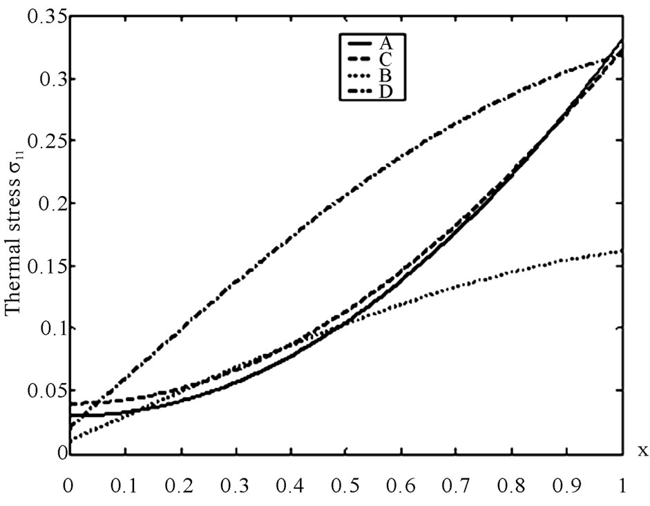
Figure 5. Variation of the thermal σ11 with x coordinate.
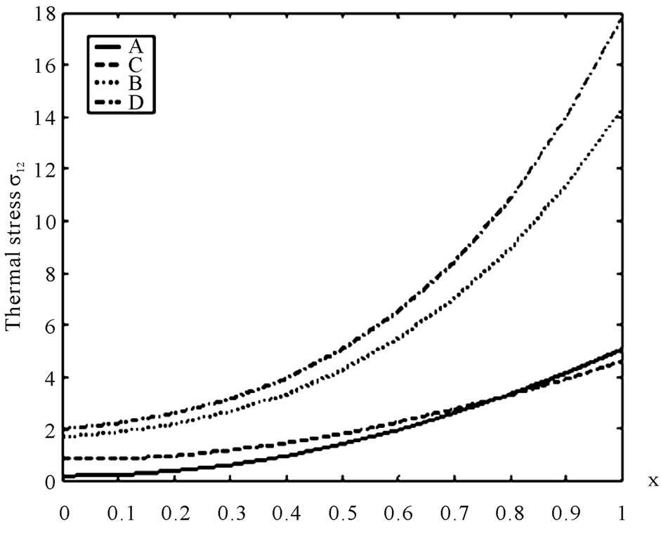
Figure 6. Variation of the thermal σ12 with x coordinate.
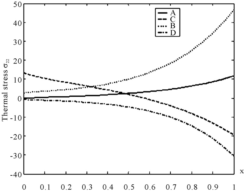
Figure 7. Variation of the thermal σ22 with x coordinate.
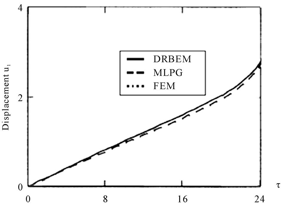
Figure 8. Variation of the displacement u1 with time τ for the three methods: DRBEM, MLPG and FEM.
 and
and  are closer in the absence of initial stress than in the presence of initial stress. We may also observe from these figures that the initial stress has an important effect on the magneto-thermo-visco-elastic stresses along
  -axis through the material constants, thermal constants, magnetic constants and viscosity factor, which are essential parameters to be considered in the design of various devices. Furthermore, while there is no limitation in the solution procedure, all boundary and initial conditions are strongly satisfied.
This phenomenon gives clear evidence of a magnetothermostress-focusing effect in a non-homogeneous anisotropic initially stressed viscoelastic solid. From this knowledge of the variation of magneto-thermo-viscoelastic stresses along  -axis in a non-homogeneous anisotropic initially stressed viscoelastic solid placed in a constant primary magnetic field, we can design various viscoelastic solids under magnetothermal load to meet specific engineering requirements and utilize it in measurement techniques of thermoviscoelasticity.
5. Conclusions
The purpose of this paper is to investigate the transient magneto-thermo-visco-elastic stresses in a non-homogeneous anisotropic body. A development of the dual reciprocity boundary element method for solving the system of fundamental equations is presented. In the case of plane deformation, a numerical scheme for the implementation of the method is presented and the numerical computations are carried out for the temperature, displacement components and thermal stress components. The validity of DRBEM is examined by considering a magneto-thermo-visco-elastic solid occupies a rectangular region and excellent agreement is obtained with existent results. The results obtained are presented graphically to show the effects of inhomogeneity and initial stress on the displacement components and thermal stress components.
REFERENCES
- A. M. El-Naggar, A. M. Abd-Alla and M. A. Fahmy, “The Propagation of Thermal Stresses in an Infinite Elastic Slab,” Applied Mathematics and Computation, Vol. 157, No. 2, 2004, pp. 307-312. doi:10.1016/j.amc.2003.08.116
- A. M. El-Naggar, A. M. Abd-Alla, M. A. Fahmy and S. M. Ahmed, “thermal Stresses in a Rotating Non-Homogeneous Orthotropic Hollow Cylinder,” Heat and Mass Transfer, Vol. 39, No. 1, 2002, pp. 41-46. doi:10.1007/s00231-001-0285-4
- C. A. Brebbia and D. Nardini, “Dynamic Analysis in Solid Mechanics by an Alternative Boundary Element Procedure,” International Journal of Soil Dynamics and Earthquake Engineering, Vol. 2, No. 4, 1983, pp. 228- 233. doi:10.1016/0261-7277(83)90040-2
- L. C. Wrobel and C. A. Brebbia, “The Dual Reciprocity Boundary Element Formulation for Nonlinear Diffusion Problems,” Computer Methods in Applied Mechanics and Engineering, Vol. 65, No. 2, 1987, pp. 147-164. doi:10.1016/0045-7825(87)90010-7
- P. W. Partridge, C. A. Brebbia and L. C. Wrobel, “The Dual Reciprocity Boundary Element Method,” Computational Mechanics Publications, Southampton, 1992.
- E. A. Divo and A. J. Kassab, “Boundary Element Methods for Heat Conduction: With Applications in Non-Homogeneous Media,” WIT Press, Southampton, 2003.
- L. Gaul, M. Kögl and M. Wagner, “Boundary Element Methods for Engineers and Scientists,” Springer-Verlag, Berlin, 2003.
- T. Matsumoto, A. Guzik and M. Tanaka, “A Boundary Element Method for Analysis of Thermoelastic Deformations in Materials with Temperature Dependent Properties,” International Journal for Numerical Methods in Engineering, Vol. 64, No. 11, 2005, pp. 1432-1458. doi:10.1002/nme.1412
- M. A. Fahmy, “Thermoelastic Stresses in a Rotating Nonhomogeneous Anisotropic Body,” Numerical Heat Transfer, Part A: Applications, Vol. 53, No. 9, 2008, pp. 1001- 1011. doi:10.1080/10407780701789179
- M. A. Fahmy, “Application of DRBEM to Non-Steady State Heat Conduction in Non-Homogeneous Anisotropic Media under Various Boundary Elements,” Far East Journal of Mathematical Sciences, Vol. 43, 2010, pp. 83-93.
- M. A. Fahmy, “A Time-Stepping DRBEM for the Transient Magneto-Thermo-Visco-Elastic Stresses in a Rotating Non-Homogeneous Anisotropic Solid,” Engineering Analysis with Boundary Elements, Vol. 36, 2012, pp. 335-345. doi:10.1016/j.enganabound.2011.09.004
- G. Davì and A. Milazzo, “A Regular Variational Boundary Model for Free Vibrations of Magneto-Electro-Elastic Structures,” Engineering Analysis with Boundary Elements, Vol. 35, No. 3, 2011, pp. 303-312. doi:10.1016/j.enganabound.2010.10.004
- M. A. Fahmy and T. M. El-Shahat, “The Effect of Initial Stress and Inhomogeneity on the Thermoelastic Stresses in a Rotating Anisotropic Solid,” Archive of Applied Mechanics, Vol. 78, No. 6, 2008, pp. 431-442. doi:10.1007/s00419-007-0150-0
- C. A. Brebbia, J. C. F. Telles and L. Wrobel, “Boundary Element Techniques in Engineering,” Springer-Verlag, New York, 1984.
- P. W. Partridge and L. C. Wrobel, “The Dual Reciprocity Boundary Element Method for Spontaneous Ignition,” International Journal for Numerical Methods in Engineering, Vol. 30, No. 5, 1990, pp. 953-963. doi:10.1002/nme.1620300502
- D. Nardini and C. A. Brebbia, “A New Approach to Free Vibration Analysis Using Boundary Elements,” In: C. A. Brebbia, Ed., Boundary Element Methods, Springer-Verlag, Berlin, 1982, pp. 312-326.
- E. L. Albuquerque, P. Sollero and M. H. Aliabadi, “Dual Boundary Element Method for Anisotropic Dynamic Fracture Mechanics,” International Journal for Numerical Methods in Engineering, Vol. 59, No. 9, 2004, pp. 1187-1205. doi:10.1002/nme.912
- H. A. Cho, M. A. Golberg, A. S. Muleshkov and X. Li, “Trefftz Methods for Time Dependent Partial Differential Equations,” CMC―Computers, Materials & Continua, Vol. 1, 2004, pp. 1-37.
- M. Guiggiani and A. Gigante, “A General Algorithm for Multidimensional Cauchy Principal Value Integrals in the Boundary Element Method,” Journal of Applied Mechanics, ASME, Vol. 57, 1990, pp. 906-915. doi:10.1115/1.2897660
- V. Mantič, “A New Formula for the C-Matrix in the Somigliana Identity,” Journal of Elasticity, Vol. 33, 1993, pp. 191-201. doi:10.1007/BF00043247
- G. H. Golub and C. F. Van Loan, “Matrix Computations,” North Oxford Academic, Oxford, 1983.
- K. J. Bathe, “Finite Element Procedures,” Prentice-Hall, Englewood Cliffs, 1996.
- N. Ahmed, “Visco-Elastic Boundary Layer Flow Past a Stretching Plate and Heat Transfer with Variable Thermal Conductivity,” World Journal of Mechanics, Vol. 1, No. 3, 2011, pp. 15-20. doi:10.4236/wjm.2011.12003
- S. Kanaun, “An Efficient Numerical Method for Calculation of Elastic and Thermo-Elastic Fields in a Homogeneous Medium with Several Heterogeneous Inclusions,” World Journal of Mechanics, Vol. 1, No. 2, 2011, pp. 31-43. doi:10.4236/wjm.2011.12005
- M. D. Monsia, “A Simplified Nonlinear Generalized Maxwell Model for Predicting the Time Dependent Behavior of Viscoelastic Materials,” World Journal of Mechanics, Vol. 1, No. 3, 2011, pp. 158-167. doi:10.4236/wjm.2011.13021
- A. M. Abd-Alla, T. M. El-Shahat and M. A. Fahmy, “Thermoelastic Stresses in Inhomogeneous Anisotropic Solid in the Presence of Body Force,” International Journal of Heat & Technology, Vol. 25, No. 1, 2007, pp. 111-118.
- A. M. Abd-Alla, M. A. Fahmy and T. M. El-Shahat, “Magneto-Thermo-Elastic Stresses in Inhomogeneous Anisotropic Solid in the Presence of Body Force,” FarEast Journal of Applied Mathematics, Vol. 27, No. 3, 2007, pp. 499-516.
- A. M. Abd-Alla, M. A. Fahmy and T. M. El-Shahat, “Magneto-Thermo-Elastic Problem of a Rotating NonHomogeneous Anisotropic Solid Cylinder,” Archive of Applied Mechanics, Vol. 78, No. 2, 2008, pp. 135-148. doi:10.1007/s00419-007-0147-8
- J. Sladek, V. Sladek, P. Solek and Ch. Zhang, “Fracture Analysis in Continuously Nonhomogeneous MagnetoElectro-Elastic Solids under a Thermal Load by the MLPG,” International Journal of Solids and Structures, Vol. 47, No. 10, 2010, pp. 1381-1391. doi:10.1016/j.ijsolstr.2010.01.025