World Journal of Mechanics
Vol. 1 No. 3 (2011) , Article ID: 5774 , 6 pages DOI:10.4236/wjm.2011.13015
Asymptotic Expansion of Temperature Close to a Singularity of a Plate
Laboratoire de Génie Civil, Université de Reims Champagne Ardenne, Moulin de la Housse, Reims, France
E-mail: isabelle.titeux@univ-reims.fr
Received March 22, 2011; revised April 21, 2011; accepted May 5, 2011
Keywords: Thin Plate, Boundary Layers, Singularities, Asymptotic Expansion
ABSTRACT
The thermal conduction in a thin laminated plate is considered here. The lateral surface of the plate is not regular. Consequently, the boundary of the middle plane admits a geometrical singularity. Close to the origin, the lateral edge forms an angle. We shall prove that the classical bidimensional problem associated with the thin plate problem is not valid. In this paper, using the boundary layer theory, we describe the local behavior of the plate, close to the perturbation.
1. Introduction
A thin plate is a three dimensional body, a dimension of which (the thickness) is smaller than the other dimensions. Usually, under the assumption of small thickness with respect to the characteristic length of the middle plane, instead of a three-dimensional description, a bi-dimensional one is used. The problem is then posed over the middle plane of the plate. In this way, the numerical methods are less expensive in time and in memory.
In this paper, we deal with the modelling of the thermal behavior of a thin laminated plate. The thermal conductivity can be considered as an exemplary problem similar to the elasticity problem. Instead of displacement, the unknown is the temperature, but the equations are similar.
The temperature and thermal flux established by the asymptotic expansion are good approximations. But close to the lateral surface, the bi-dimensional behavior is not suited: for a laminated body, boundary conditions are only satisfied on average. However, on the edge damage phenomena can appear, like delamination, crack... A bi-dimensional description of the behavior of the plate is not enough. In order to predict these phenomena, we need a good, local description of the behavior of the plate, in these areas. In this case, the bi-dimensional expansion is no more sufficient, we need a local three-dimensional description, which is valid only close to the lateral surface. Moreover, the distance to the edge and the position in the thickness have the same range of magnitude; the assumption of small thickness with respect to the other directions is no more valid. Close to the edge, the body must be considered like a threedimensional domain, with thickness and distance to the edge of the same order.
In previous works, the cases of a classical regular edge [1] and edge with a local perturbation [2] were considered. Recently, Saidi et al. [3,4] studied singularities in the edge of moderately thick plates. They studied the effect of the boundary layer term added to the Mindlin’s plate theory. In this paper, the case of thin laminated plate with an angle in the lateral edge is considered. We lose the symmetry of the local perturbation [2] and new arguments must be used. Because of this angle, the boundary of the plate cannot be considered as a smooth surface. The boundary layer theory must be adapted to take into account the new geometry of the perturbed edge. Therefore, we obtain a new local description which is posed on an unbounded domain. The existence and uniqueness of the solution must be proved in order to implement a numerical method of resolution.
2. Generalities and Description of a Thin Laminated Plate
2.1 Classical Problem for a Thin Plate
Insert Figure 1: The plate 
Let us consider a thin plate  characterized by its middle plane
  and its thickness
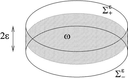
Figure 1. The plate .
.
 (cf. Figure 1). In fact,
  denotes the ratio between the characteristic length of the middle plane of the plate and the thickness. Let
  and
and  denote the upper and lower faces respectively and
  denotes the lateral edge.
Coordinates in the middle plane are  and position in the thickness is
 . Symbols in boldface denote vectors. We use the summation convention on repeated indices. Lati
 n indices take their values in the set
  while Greek ones take their values in the set
 .
.
For given external sources of heat, we have to determine the temperature field . The thermal flux vector is related to
  by the constitutive law
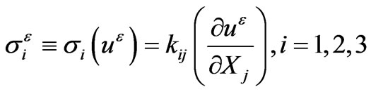
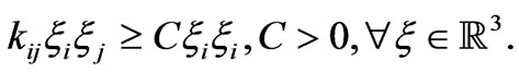
The coefficients are the conductivity coefficients. They satisfy symmetry and coerciveness properties:

The equilibrium equation is
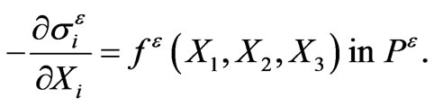 (2.1)
(2.1)
The order of magnitude of  is
is  it means that
  has the same order than the characteristic length of the middle plane. The upper and lower faces of the plate are free of heat source
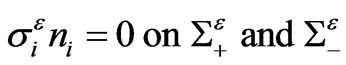 (2.2)
(2.2)
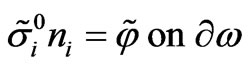
On the lateral edge of the plate, there are Neumann's boundary conditions:
 (2.3)
(2.3)
where  is
is  and n is the outer normal.
The external sources of heat satisfy the compatibility condition

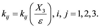
The plate is laminated, i.e. composed of several materials. We assume that the interfaces between two materials are parallel to the middle plane of the plate. In this way, the conductivity coefficients depend on the position in the thickness , we assume that they do not depend on the other variables:
At the interface between two different materials, the temperature and the normal thermal flux are continuous:
 (2.4)
(2.4)
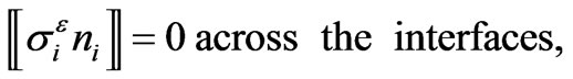 (2.5)
(2.5)
where the brackets denote the jump across the interfaces.
Problem (2.1)-(2.5) is the plate problem.
Remark 1. In (2.1) and (2.3), external sources of heat are taken with an order of magnitude of 1 in order to get an asymptotic expansion of the solution with the leading term  (see (2.7) thereafter). But, because of the linearity of the problem, if the external sources of heat are multiplied by a constant (even depending on
 ), the solution is also multiplied by the same constant.
Using the change of variables
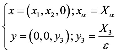 (2.6)
(2.6)
the asymptotic expansion theory [5,6] involves temperature of the form
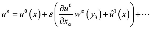 (2.7)
(2.7)
The functions  only depend on the conductivity coefficients; they are solutions of the variational problems

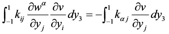
where .
.
The change of variables (2.6) is equivalent to dilate the thickness of the plate. In this way, we obtain a new plate  which does not depend on
  (cf. Figure 2). All the directions of the plate have now the same range of magnitude. The thickness of
  is no more small with respect to the other directions. We shall denote by
 and
and  the upper and lower faces of the plate
 , and by
  the lateral edge.
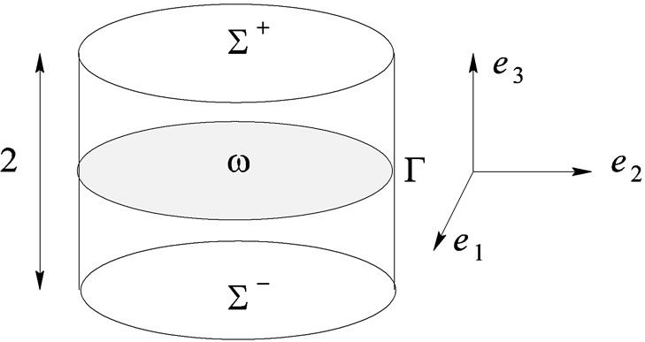
Figure 2. The plate .
.
Insert Figure 2 The plate .
.
Let us remind certain features of the asymptotic structure of the plate problem [5,6]. The asymptotic structure of the mean value of the thermal flux is of the form:

where the tilde denotes the average on the thickness and  is the leading term of the thermal flux. The homogenized conductivity coefficients are given by
 ,
,
 The problem for
 is posed over the middle plane. So that it is a bi-dimensional problem
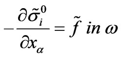 (2.8)
(2.8)
 (2.9)
(2.9)
where  and
and  are the leading terms of
  and
and  respectively.
If the plate is laminated, it means that the plate is not homogeneous. Equations (2.3) and (2.9) are not equivalent: the mean value is different from the value on each point of the lateral surface. Consequently, the asymptotic solution is not valid everywhere on the plate. Close to the edge, a corrective term must be added.
2.2 Behavior of the Thin Plate Close to a Classical edge
It can be important to have a good approximation of the boundary of the plate, if for instance the damage is studied. As a matter of fact the cracks appear on the edge, like delamination. In this case, a local three-dimensional description of the behavior of the plate is necessary.
On the lateral edge the assumption of very small  with respect to the other variables is not justified. Distance to the edge is of the same range of magnitude than the thickness of the plate.
Insert Figure 3 The specific directions.
In order to study the temperature close to the edge, let us define local axes  (cf. Figure 3):
  is the tangent direction of the edge of the middle plane
 ,
,  is normal to
  in the middle plane, pointing inside
 ,
,  is normal to
 .
.
A corrective term is added to the asymptotic expansion of the temperature [1] to improve it. In order to act on the leading term of the thermal flux, we have to correct the second term of the temperature. As a matter of fact, if we act on the first term , we shall change the order of the thermal flux.
Let  be the corrective term of the temperature, the new asymptotic expansion close to the edge is
 (2.10)
The corrective term must depend on the position in the thickness  and on the distance to the lateral edge
 . The position on the edge
  is a parameter. So that, it is defined in a semi infinite strip,
 (2.11)
It can be proved [6] that  is the unique solution of the variational problem


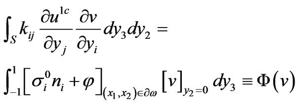 (2.12)
where  is the completed space of
  for the norm associated with
 (2.13)

Figure 3. The specific directions.
The separation of variables method [6,7], allows to assume that the corrective term decreases exponentially.
3. Boundary Layer Close to an Angle
As it was seen in subsection 2.2, the corrective term allows to improve the description of the thermal flux close to a regular edge of the plate. In the same way, the behavior of the plate close to an angle, can be given by an asymptotic expansion with a new corrective term, a new boundary layer term.
Now, the boundary of the plate is not regular, it admits a perturbation. Close to the origin, the edge forms an angle of magnitude  (cf.Figure 4). The middle plane of the plate is no more regular. The lateral edge
  can be split into two parts:
  and
and .
.
Figure 4 The perturbation of the edge In order to lighten the notations, we shall assume that  vanishes in the vicinity of the origin.
The edge is assumed to be regular everywhere but not in the vicinity of the origin.
Far from the origin, but on the lateral edge, the boundary layer problems are similar to those described in section 2, corresponding to a classical, regular surface.
Let  denotes the corrective term on
  far from the origin. In the same way, let
  denotes the corrective term on
  far from the origin. These functions
 ,
,  , are solutions of the variational problem (2.12) with unknown
  instead of
 .
.
We can also prove that they are solutions of
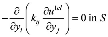 (3.1)
(3.1)
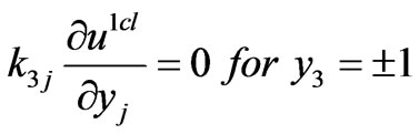 (3.2)
(3.2)
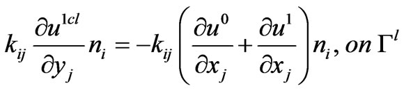 (3.3)
(3.3)
 (3.4)
(3.4)
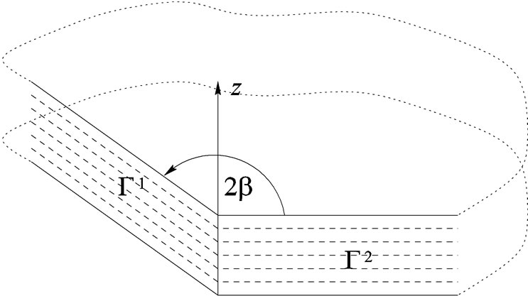
Figure 4. The perturbation of the edge.
 (3.5)
(3.5)
 (3.6)
(3.6)
where  is defined in (2.11).
Close to the origin, a corrective term,  is added to
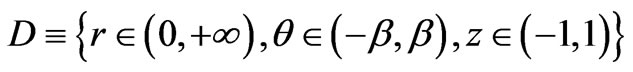
  in the asymptotic expansion (2.7). It depends on the three space components. It is defined in an unbounded domain
  which is the dilatation of the origin. As a matter of fact, close to the origin, all directions (the position in the thickness and the distance to the origin) have the same range of order. Because of the geometry of the domain, it will be useful to introduce the cylindric coordinates to describe the domain:
 .
.
The asymptotic expansion of the temperature is now

where the unknown is .
.
When , the boundary condition (2.3) must be exactly satisfied at the corresponding order. When
  becomes great, the corrective term must tend to the classical boundary layer term. We shall gather
  and
and  into a unique function
  defined by
Remark 2. For small values of  and great values of
 , it means far from the lateral edge, the influence of each corrective term
  is very small because of the exponentially decreasing. So that they can be neglected.
We can then see that, because  is unbounded, and because the corrective term must tend to
  when
when  becomes great, it cannot belong to
  We shall transform the corrective term in order to obtain an unknown which belongs to
 . Let us define:

where the new unknown is now .
.
The function , which is
 , is a cut off function such that for little
  is equal to 0 and for great value of
  is equal to 1 (cf. Figure 5).
insert figure 5 The cutoff function 
The problem for  is now:
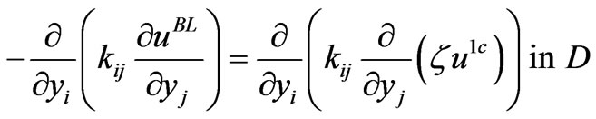 (3.7)
(3.7)

Figure 5. The cutoff function 
 (3.8)
(3.8)
 (3.9)
(3.9)
 (3.10)
 (3.11)
 (3.12)
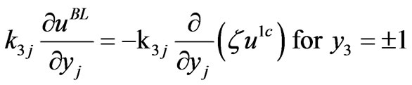
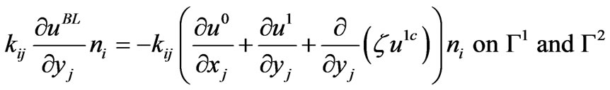
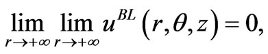
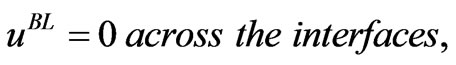
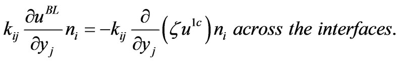
Equation (3.7) is the equilibrium equation, (3.8) is the boundary condition on  and
and , (3.11) and (3.12) are the continuity conditions across the interfaces, (3.9) is the boundary condition on the lateral edge, and (3.10) means that the corrective term is inefficient far from the origin.
Remark 3. When  is sufficiently great,
  is equal to 1 and the right-hand sides of (3.7), (3.8), (3.9) and (3.12) vanish.
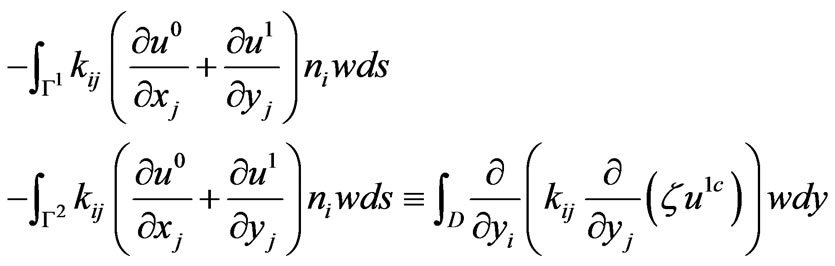
Problem (3.7)-(3.12) is equivalent to the following variational problem:
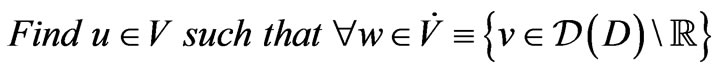
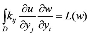 (3.13)
With


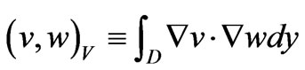
Where  is the completed space of
  for the norm associated with
Lemma 1. The right-hand side of (3.13) is a functional over .
.
Proof.  is defined over a space of equivalent classes. Two elements of a same class differ by a constant. It follows that
  is a functional over
  if two elements of a same class take the same value by
 , or if, for any constant
 ,
, . Using the first expression of
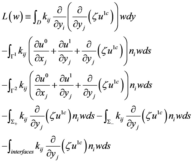
  in (3.14), we get
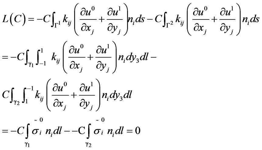
by virtue of (2.9) and the assumption on .
.
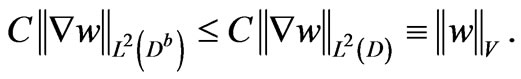
Lemma 2. The functional  is bounded over
 . It means that there exists a constant
  such that for all
 ,
, .
.
Proof. Let  be any element of
 , using the second expression of
  in (3.14)
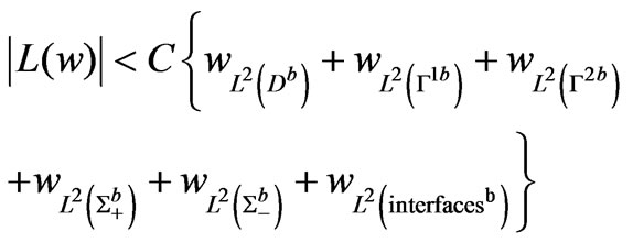
By virtue of remark 3 each integral can be applied on a bounded domain which does not depend on . As a consequence,
  can be read

where the upper-script  means that the domain is bounded. Using the Cauchy-Schwarz inequality,
Using the trace theorem and because  is a bounded domain, we get

Passing to the quotient space 
 but
but
Because of the density of  into
into , Equation (3.13) is valid in the whole
 . It follows from the Lax-Milgram theorem, lemma 2 that Theorem. The corrective term
  is uniquely defined over
 .
.
4. Conclusions
In order to improve the description of the behavior of the plate close to the singularity, a boundary layer term was added. This term is solution of (3.7)-(2.12). It has no influence far from the edge but it is defined over an unbounded domain.
At first, the equivalent variational problem was found. Then, the previous theorem allows us to prove the existence and the uniqueness of the solution. In this way the numerical resolution can be implement.
REFERENCES
- H. Dumontet, “Homogénéisation et Effets de Bords dans les Matériaux Composites,” Ph. D. Thesis, Paris, 1990.
- I. Titeux, “Problèmes de Fracture et Comportement Local Pour les Plaques Composites Anisotropes,” Ph. D. Thesis, Paris, 1995.
- A. R. Saidi, F. Hejripour and E. Jomehzadeh, “On the Stress Singularities and Boundary Layer in Moderately Thick Functionally Graded Sectorial Plates,” Applied Mathematical Modelling, Vol. 34, No. 11, 2010, pp 3478-3492. doi:10.1016/j.apm.2010.02.036
- E. Jomehzadeh and A. R. Saidi, “Analytical Solution for Free Vibration of Transversely Isotropic Sector Plates Using a Boundary Layer Function,” Thin Walled Structures, Vol. 47, No. 1, 2009, pp. 82-88. doi:10.1016/j.tws.2008.05.004
- J. Sanchez-Hubert and E. Sanchez-Palencia, “Introduction Aux Methods Asymptotiques et à L'homogénéisation,” Masson, Paris, 1992.
- D. Leguillon and E. Sanchez-Palencia, “Computation of Singular Solutions in Elliptic Problems and Elasticity,” Masson, Paris, 1988.
- I. Titeux and Y. Yakubov, “Completeness of Root Functions for Thermal Conduction in a Strip with Piecewise Continuous Coefficients,” Mathematical Models and Methods in Applied Sciences, Vol. 7, No. 7, 1997, pp. 1035-1050.