World Journal of Condensed Matter Physics
Vol. 3 No. 4 (2013) , Article ID: 38337 , 5 pages DOI:10.4236/wjcmp.2013.34030
Spin Configurations in the Rectangular Lattice
![]()
Department of Physics, Selcuk University, 42075 Campus, Konya, Turkey.
Email: *gmert@selcuk.edu.tr
Copyright © 2013 Gulistan Mert, Hasan Sevki Mert. This is an open access article distributed under the Creative Commons Attribution License, which permits unrestricted use, distribution, and reproduction in any medium, provided the original work is properly cited.
Received July 30th, 2013; revised September 6th, 2013; accepted September 17th, 2013
Keywords: Spin Configuration; Exchange Interaction; Magnetic Mode; Magnetic Structure
ABSTRACT
Using matrix method, the possible spin configurations have been determined for four sublattices in rectangular lattice taking into account only nearest-neighbor exchange interactions. We obtain collinear and non-collinear spin configurations in the ground and the first excited states for the three different propagation vectors. When k = 0, depending on the sign of exchange parameters, we find a ferromagnetic mode and three antiferromagnetic modes. When k = [1, 1] and [1.5, 1.5], we find non-collinear (canted) spin configurations. Moreover, we observe that spins of some sublattices in the excited state change their orientations.
1. Introduction
Bertaut’s matrix method enables possible magnetic modes associated with a given propagation vector in magnetic systems [1-3]. The symmetry properties of crystal gain importance. Moreover, method is valid for magnetic cells different from the chemical cells. For Bravais lattice, it reduces to Villain’s method [4]. From the other part, the results of this method are also agreed with that of group theory. The greatest advantage of this method is to consider fundamental interaction being isotropic classical Heisenberg and is also applicable when the chemical and magnetic cells are not identical. Moreover, isotropic terms as well as anisotropic terms can be expressed by a Hamiltonian of a second order and problem can be reduced to an eigenvalue problem. Solving this eigenvalue equation, one is able to find all possible magnetic config- urations. Townsend et al. dealt with triangular-spin structure by the application of this method and predicted triangular-spin magnetic ordering for KFe3(OH)6(SO4)2 and KFe3(OH)6(CrO4)2 [5]. Macroscopic (group theoretical) and microscopic (matrix) methods were applied to the two-dimensional orthorhombic lattice with four spins by Darendelioğlu et al. and they determined that the four collinear modes are along the z-axis and the non-collinear modes are in the xy-plane of the two-dimensional orthorhombic lattice [6]. Belorizky performed a systematic research of the bilinear exchange Hamiltonian providing a ground state spin configuration for two and three dimensional lattices [7]. Yu et al. have given the phase diagram of the different spin configurations of a magnetic bilayer system consisting of two ferromagnetic layers, based on a phenomenological model [8]. On the other hand, many researchers studied experimentally whether colinear and non-collinear structures exist in DyNiC2 and HoNiC2 compounds [9], in Mn5Ge3 compound [10], in La1.5Sr0.5CoO4 [11] and in ɛ-FexN [12].
In this paper, we will apply the Bertaut’s matrix method to the four-sublattice model in rectangular lattice for the given propagation vectors in the ground and the first excited states as taking only nearest-neighbor exchange interaction. The outline of this paper is as follows. In Section 2, we follow the matrix method of Bertaut and give the fundamental equations. In Section 3, we have determined possible spin configurations depending on the propagation vectors and the sign of exchange parameters and found collinear and non-collinear (canted) spin configurations. Finally, Section 4 contains conclusions.
2. Matrix Method
We derive spin configurations of the four sublattices on rectangular lattice using the Bertaut’s matrix method [2]. We will assume that there is a classical interaction of Heisenberg type between the nearest-neighbor spins. Hamiltonian is given by
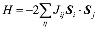 , (1)
, (1)
where Jij is the exchange integral between spins at ri and rj. Si is the spin at point ri.
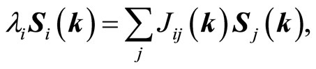
Using the translational symmetry of the system, one obtains:
 (2)
(2)
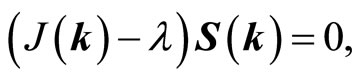
where λi is a constant of proportionality, having the dimension of an energy. After a Fourier transformation, Equation (2) can be written as matrix equation:
 (3)
(3)
where λ is the diagonal matrix formed by the elements λiδij ( ; n is the number of sublattices). Si(k) is a column vector being the Fourier transformations of the Si(ri):
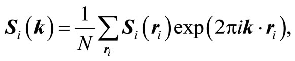 (4)
(4)
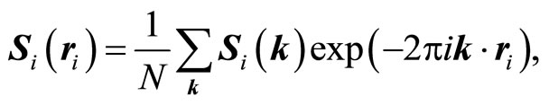 (5)
(5)
where N is the number of unit cells in the lattice. The hermitian interaction matrix J(k) is Fourier transformation of Jij and whose matrix elements are defined as follows:
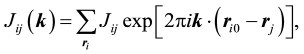 (6)
(6)
where ri0 is a fixed reference point and the summation is over all rj belonging to the same Bravais lattice j.
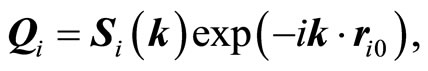
The expression of Si(k) depended on phase is given by:
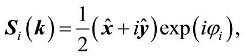 (7)
(7)
where  and
and  are orthogonal unit vectors,
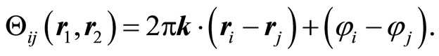
  is the phase angle of sublattice i. The angle between two spins Si(ri) and Si(ri) in a one mode solution is given by
 (8)
(8)
The matrix J(k) in Equation (3) still depends on the atomic coordinates. With following transformation of eigenvectors
 (9)
(9)
one may construct a hermitian matrix η(k) which does not depend on the atomic coordinates:
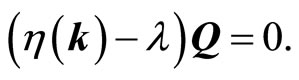 (10)
(10)
η(k) matrix elements contain Fourier transform of the exchange integrals between ions occupying the sublettices.
In the case of only one propagation vector k, the reference spins are simply given by
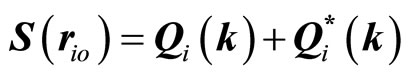 (11)
(11)
 (12)
(12)
 (13)
(13)
This equation is the main equation in order to find spin directions for the given k-vectors.
3. Results and Discussions
We consider the four magnetic ions (labeled as 1, 2, 3 and 4) localized rectangular lattice displayed in Figure 1 in which one shows also the corresponding exchange integrals. The ions occupy the positions: 1) x, y; 2) x, –y; 3) –x, –y; 4) –x, y. Our exchange integrals J1, J2 and J3 correspond to ,
,  and
and , respectively. For this specific case, we have taken the exchange parameters as follows: J1 = 0.05, J2 = 0.001 and J3 = 0.02 or J1 = –0.05, J2 = –0.001 and J3 = –0.02.
Our interaction matrix has the form
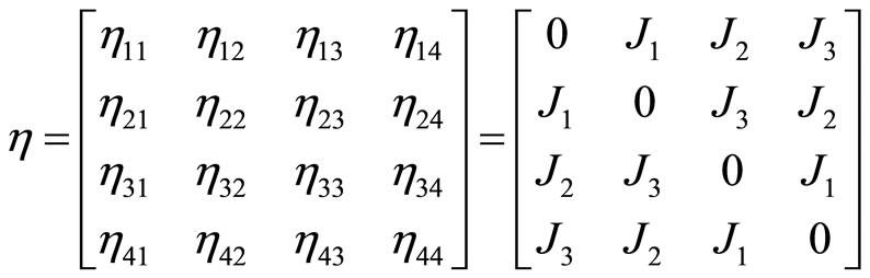 (14)
(14)
We have to find the eigenvectors and eigenvalues of the matrix in Equation (14). The solution to this homogenous equations system depends on the satisfaction of the following condition:
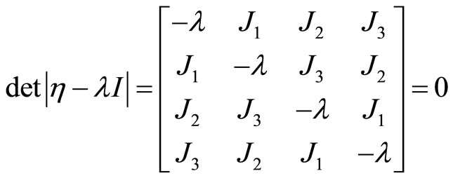 (15)
(15)
We have determined numerically eigenvalues li (i = 1, 2, 3, 4) and corresponding eigenvectors. The stability conditions of the calculated modes follow from the condition that l must be a maximum (The quadratic form the coefficients of which are the second derivates of -l must be definite positive).
The obtained eigenvalues and eigenvectors are displayed at Table 1 for the positive and negative values of exchange parameters and given k-vectors. The phase angles of four sublattices in the ground and the first excited state for the positive and negative values of exchange parameters are displayed at Table 2.
Using the k-vectors and the phase angles, given at Table 2, in the expression for Si(ri, 0), we obtain the orientation of every spin vectors and possible spin configurations in the ground and first excited state. The obtained
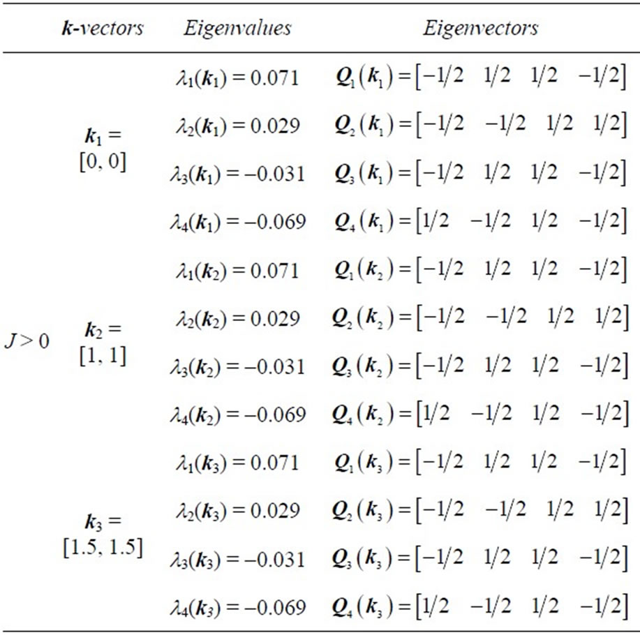
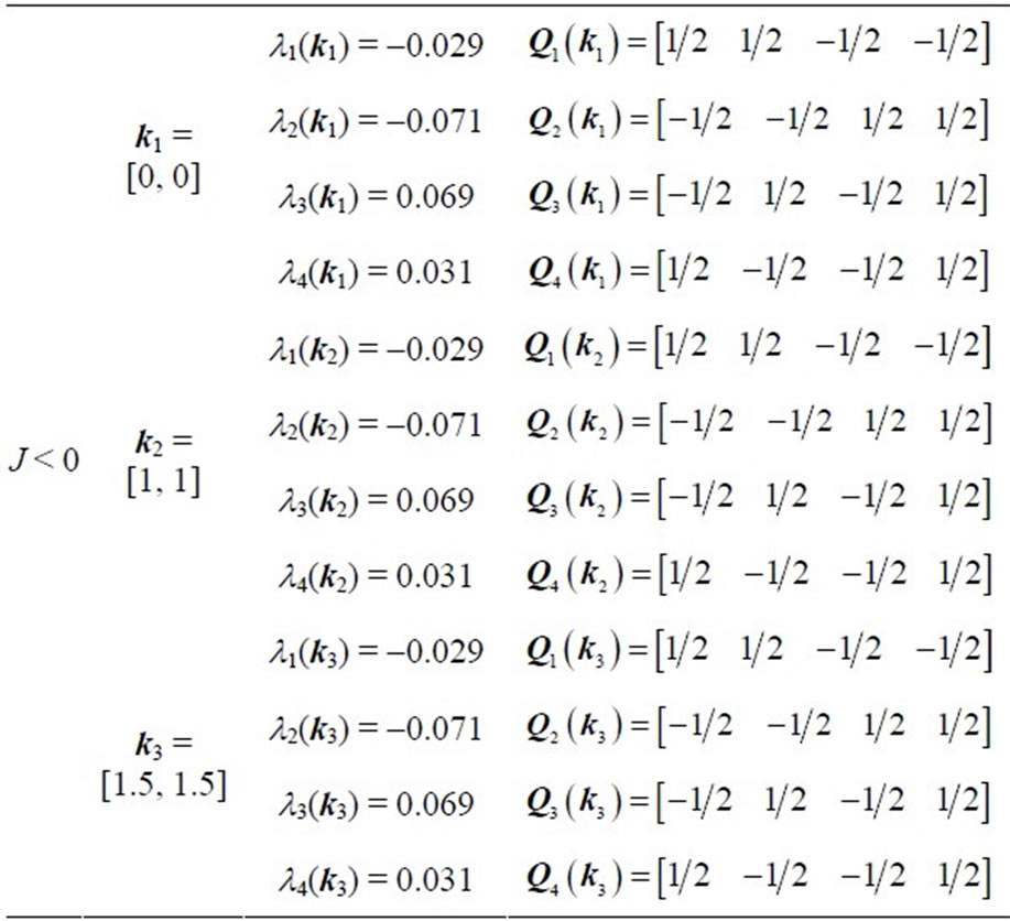
Table 1. Computationally obtained eigenvelues and their eigenvectors for given k-vectors and the positive and negative values of exchange parameters.
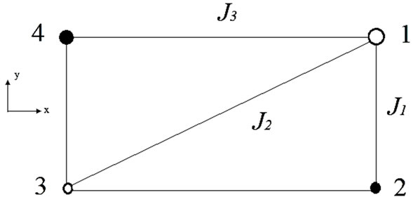
Figure 1. The rectangular lattice with the four sublattices and the magnetic interactions between neighboring ions.
results are displayed in Figures 2, 3 and 4.
Figure 2 shows the spin configurations of the ground and the first excited state for the positive and negative values of exchange parameters when k1= [0, 0]. As it is seen by the figure, spin configurations have collinear
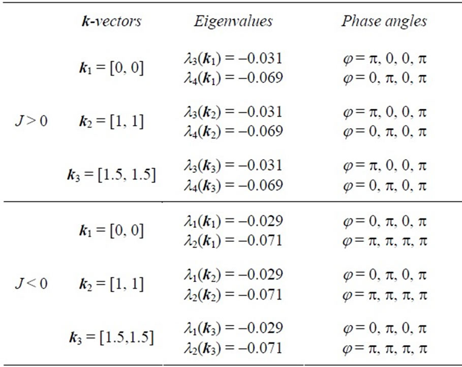
Table 2. The corresponding phase angles in the ground and the first excited states the positive and negative values of exchange parameters.
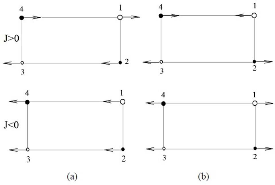
Figure 2. Spin configurations for the propagation vector k1 = [0, 0] (a) in the ground state (b) in the first excited state.
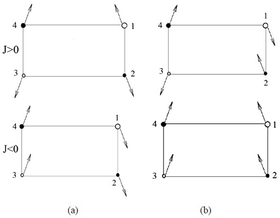
Figure 3. Spin configurations for the propagation vector k2 = [1, 1] (a) in the ground state (b) in the first excited state.
structure. They have a ferromagnetic and three antiferromagnetic structures. Belorizky et al. consider a simple
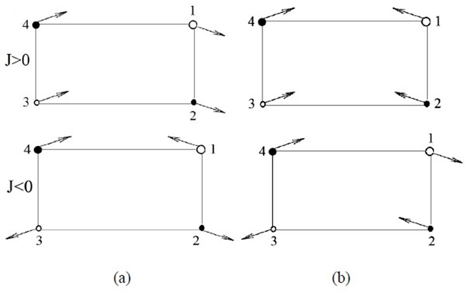
Figure 4. Spin configurations for the propagation vector k3 = [1.5, 1.5] (a) in the ground state (b) in the first excited state.
cubic lattice and find a ferromagnetic and three antiferromagnetic spin configurations at T = 0 K [13]. That the propagation vector of the configuration is zero means that in this configuration magnetic and chemical cells are identical. It is observed that spins of the sublattices 1 and 2 in the excited state have changed their orientations. Moreover, spins of the sublattices 1 and 2 in the case of J < 0 have changed their orientations.
Figure 3 shows the spin configurations of the ground and the first excited state for the positive and negative values of exchange parameters when k2 = [0.5, 0.5]. We have non-collinear spin configurations (canted) spin configurations.
As it is seen from figure, one observes that spins of the sublattices 1 and 2 in the excited state have changed their orientations. Moreover, spins of the sublattices 1 and 3 in the case of J < 0 have changed their orientations.
Figure 4 shows the spin configurations of the ground and the first excited state for the positive and negative values of exchange parameters when k2 = [1.5, 1.5]. Spin behaviors are similar to Figure 3 but their angles are different.
4. Conclusion
The Bertaut’s Matrix method is applied to rectangular lattice with the four sublattices as taking only nearestneighbor exchange interaction. For certain values of these exchange parameters, the energies are obtained as a function of k. For every k-vector the corresponding eigenvectors are also obtained and the phase angles of these sublattices are calculated for the ground and the first excited states. Finally, using the phase angles, the orientations and configurations of spins are determined. When k = 0, depending on the sign of exchange parameters, we found a ferromagnetic mode and three antiferromagnetic modes. When k = [1, 1] and [1.5, 1.5], we found non-collinear (canted) spin configurations. It is observed that spins of some sublattices in the excited state have changed their orientations.
REFERENCES
- E. F. Bertaut, “Configurations de Spin et Théorie des Groups,” Journal de Physique et le Radium, Vol. 22, No. 5, 1961, pp. 321-322. http://dx.doi.org/10.1051/jphysrad:01961002205032100
- E. F. Bertaut, “Lattice Theory of Spin Configuration,” Journal of Applied Physics, Vol. 33, No. 3, 1962, pp. 1138-1143. http://dx.doi.org/10.1063/1.1728635
- A. Kallel, H. Boller and E. F. Bertaut, “Helimagnetism in MnP-Type Compounds: MnP, FeP, CrAs and CrAs1−xSbx Mixed Crystals,” Journal of Physics and Chemistry of Solids, Vol. 35, No. 9, 1974, pp. 1139-1152. http://dx.doi.org/10.1016/S0022-3697(74)80132-0
- J. Villain, “La Structure des Substances Magnetiques,” Journal of Physics and Chemistry of Solids, Vol. 11, No. 3-4, 1959, pp. 303-309. http://dx.doi.org/10.1016/0022-3697(59)90231-8
- M. G. Townsend, G. Longworth and E. Roudaut, “Triangular-Spin, Kagome Plane in Jarosites,” Physical Review B, Vol. 33, No. 7, 1986, pp. 4919-4926. http://dx.doi.org/10.1103/PhysRevB.33.4919
- H. Ş. Darendelioğlu and H. Yüksel, “Spin Configuration of Two-Dimensional Orthorhombic Lattice,” Journal of Physics and Chemistry of Solids, Vol. 54, No. 11, 1993, pp. 1599-1602. http://dx.doi.org/10.1016/0022-3697(93)90355-U
- E. Belorizky, “Exact Ground State Spin Configurations for 2D and 3D Lattices with Nearest Neighbor Bilinear Exchange,” Solid State Communications, Vol. 96, No. 11, 1995, pp. 853-858. http://dx.doi.org/10.1016/0038-1098(95)00588-9
- M. H. Yu and Z. D. Zhang, “Spin Configurations in the Absence of an External Magnetic Bilayer with in-Plane Cubic or Uniaxial Anisotropies,” Journal of Magnetism and Magnetic Materials, Vol. 195, No. 2, 1999, pp. 514- 519. http://dx.doi.org/10.1016/S0304-8853(99)00101-8
- J. K. Yakinthos, P. A. Kotsanidis, W. Schäfer, W. Kockelmann, G. Will and W. Reimers, “The Two-Component Non-Collinear Antiferromagnetic Structures of DyNiC2 and HoNiC2,” Journal of Magnetism and Magnetic Materials, Vol. 136, No. 3, 1994, pp. 327-334. http://dx.doi.org/10.1016/0304-8853(94)00306-8
- A. Stroppa and M. Peressi, “Non-Collinear Magnetic States of Mn5Ge3 Compound,” Physica Status Solidi (a), Vol. 204, No. 1, 2007, pp. 44-52. http://dx.doi.org/10.1002/pssa.200673014
- K. Horigane, T. Uchida, H. Hiraka, K. Yamada and J. Akimitsu, “Charge and Spin Ordering in La2−xSrxCoO4 (0.4 < x < 0.6),” Nuclear Instruments and Methods in Physics Research A, Vol. 600, No. 1, 2009, pp. 243-245. http://dx.doi.org/10.1016/j.nima.2008.11.141
- S. Kurian and N. S. Gajbhiye, “Non-Collinear Spin Structure of ɛ-FexN (2 < x < 3) Observed by Mössbauer Spectroscopy,” Chemical Physics Letters, Vol. 489, No. 4, 2010, pp. 195-197. http://dx.doi.org/10.1016/j.cplett.2010.02.072
- E. Belorizky, R. Caslegno and J. Sivardiare, “Configurations of a Simple Cubic Lattice of Pseudo-Spins S = 1/2 with Anisotropic Exchange,” Journal of Magnetism and Magnetic Materials, Vol. 15-18, 1980, pp. 309-310. http://dx.doi.org/10.1016/0304-8853(80)91064-1
NOTES
*Corresponding author.