Atmospheric and Climate Sciences
Vol. 2 No. 3 (2012) , Article ID: 21399 , 15 pages DOI:10.4236/acs.2012.23029
Statistical Models for Long-Range Forecasting of Southwest Monsoon Rainfall over India Using Step Wise Regression and Neural Network
1National Center for Medium Range Weather Forecasting, Noida, India
2National Climate Centre, India Meteorological Department Shivajinagar, Pune, India
343, Ritu Apartments A-4, New Delhi, India
Email: *ashok@ncmrwf.gov.in
Received January 6, 2012; revised February 10, 2012; accepted March 9, 2012
Keywords: Monsoon; ISMR; LRF; Step-Wise Regression; Neural-Networks
ABSTRACT
The long-range forecasts (LRF) based on statistical methods for southwest monsoon rainfall over India (ISMR) has been issued by the India Meteorological Department (IMD) for more than 100 years. Many statistical and dynamical models including the operational models of IMD failed to predict the operational models of IMD failed to predict the deficient monsoon years 2002 and 2004 on the earlier occasions and so had happened for monsoon 2009. In this paper a brief of the recent methods being followed for LRF that is 8-parameter and 10-parameter power regression models used from 2003 to 2006 and new statistical ensemble forecasting system are explained. Then the new three stage procedure is explained. In this the most pertinent predictors are selected from the set of all the potential predictors for April, June and July models. The model equations are developed by using the linear regression and neural network techniques based upon training set of the 43 years of data from 1958 to 2000. The skill of the models is evaluated based upon the validation set of 11 years of data from 2001 to 2011, which has shown the high skill on the validation data set. It can be inferred that these models have the potential to provide a prediction of ISMR, which would significantly improve the operational forecast.
1. Introduction
The success of agriculture in India depends primarily on the proper amount and distribution of rain during the southwest monsoon season (June-September). The mean monsoon seasonal rainfall averaged over the country as a whole is 89 cm with a coefficient of variation of about 10%. The fluctuation of this order, however not very large, can have large impacts on water levels and agriculture sector. Even though, the contribution from agriculture sector to the national income has decreased over the years (less than 30% now), the performance of the agricultural sector is still very critical to India’s economy. During the 2 years, 2002 and 2004, deficient rainfall during the south-west monsoon season has had an adverse impact on India’s economy. An accurate long range forecast of monsoon rainfall over the country as a whole is also very useful for better macro level planning of water, power and financial resources. Therefore long-range forecasting (LRF) of southwest monsoon rainfall is a high priority in India.
During the period 1924 to 1987, long-range forecasts (LRFs) for southwest monsoon rainfall were issued for NW India and peninsular India using different multiple regression models. Initially only the surface parameters were used and it was found by 1950 that performance of these models was not good. Later the upper air parameters were also used for improving the models [1,2]. Verification of these forecasts (1924-1987) revealed that about 64% of these forecasts were found to be correct. During the decade of 1981-1990, concerted efforts made to develop new LRF techniques resulted in the development of new types of LRF models, namely dynamical stochastic transfer model [3], parametric and power regression models [4,5]. During the period of 1988-2002, IMD’s operational long range forecasts were based on the 16-parameter power regression and parametric models. The parametric model is purely qualitative and it indicates whether monsoon would be normal, excess or deficient. In this model, equal weights are given to each of the 16 parameters. The power regression model is a quantitative model, which acknowledges the nonlinear interactions of different important climatic forcings with the Indian monsoon.
Statistical monsoon prediction models are based upon the strong correlations of the southwest monsoon rainfall over India (ISMR) with certain antecedent atmospheric, oceanic and land parameters. A common weakness of all statistical models is that while the correlations are assumed to remain constant in future, they may, and in fact do, change with time and slowly lose their significance. In 2003, a critical re-evaluation of the 16-parameter power regression and parametric models was made and it revealed that correlations of 10 parameters had rapidly declined in recent years. An extensive search for new parameters which are physically well-related and statistically stable leads to the identification of 4 new predictors of monsoon rainfall. This resulted in building a set of 10 stable parameters (Table 1) consisting of 6 out of the earlier 16 parameters and 4 new parameters.
Out of the above 10 parameters, 8 needed data only up to March and 2 needed data up to June. Using these 10 parameters, IMD developed two power regression (PR) models, one using 8 parameters needing data up to March and another using the full set of 10 parameters. In addition to these PR models, probabilistic models using the same 8-parameters and 10-parameters respectively were developed to issue qualitative forecast. Based on these models, a two stage forecasting system was adopted in 2003, for issuing operational forecast for press and public. The first stage LRF for the summer monsoon seasonal rainfall for the country as a whole was issued in the middle of April every year using 8-parameter PR & probabilistic models. In the next stage, LRF update for the first stage forecast was issued in the beginning of July using the 10-parameter PR & probabilistic models for the country as a whole.
In the present study a three stage procedure is followed. The non-overlapping set of 16 parameters for July forecast, 14 parameters for June forecast and 11 parameters for April forecast are considered as the set of potential predictors from these 10 + 8 parameters. Step wise regression with selection of predictors is applied for selecting the most pertinent predictors which explains most of the variance for each stage forecast. Then the models are developed based upon the selected predictors using linear regression and neural network as explained in the following sections.
2. Brief Introduction to Recent Methods Being Followed
2.1. The 8-Parameter and 10-Parameter Power Regression Models
2.1.1. Models for Seasonal Rainfall
The 8 and 10 parameter PR models were used for issuing quantitative operational forecast of seasonal rainfall over the country as a whole during the period 2003 to 2006. Table 1 shows the predictors used for the development of the PR models. The mathematical form of the power regression model is given below.
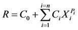
where R is the rainfall, Xs are standardized predictors, and Cs and Ps are constants. n is either 8 or 10. The model is non-linear and the power term, P, in the above equation varies between ±2.
The models were developed using data of 38 years (1958-1995) and independently tested using data of 7 years (1996-2002). A comparison of the new 8 and 10 parameter models with the earlier used 16-parameters
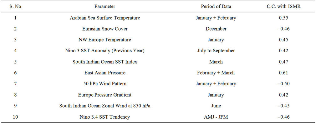
Table 1. List of 10 parameters used for developing new LRF models.
power regression model indicated that the forecasts from the 8 and 10 parameter models were closer to the actual rainfall than the forecasts from the 16 parameter model. More details of these models can be seen in [6]. However, it may be mentioned that though these models showed better performance in general they failed to correctly indicate the large rainfall deficiency during 2002 in the hindcast mode and that during 2004 in real time forecast mode.
2.1.2. Models for Probabilistic Forecast
The Probabilistic models were based on the statistical linear discriminant analysis (LDA) technique[7] and [8] and used the same sets of 8 and 10 parameters being used for the power regression models discussed above. The LDA is a useful technique to find out which predictor variables discriminate between two or more naturally occurring (or a priori defined) predictand groups. The LDA also estimate the posterior probabilities for a predictand to fall into each of these groups. The primary assumption for this model is that prior probabilities of all the predictand groups (or quints) are equal. The data for 40 years (1958-1997) were used for the model development and data for 5 years (1998-2002) were used for the model verification. The seasonal rainfall (predictand) was grouped into 5 broad categories of equal probability (20% each) i.e. each group consisted of 8 years. These categories are deficient (<90% of LPA), below normal (90% - 97% of LPA), near normal (98% - 102% of LPA), above normal (103% - 110% of LPA) and excess (>100% of LPA).
In hindcast mode, the 8 parameter LDA model showed 68% correct classifications, whereas the 10 parameter LDA model showed 78% correct classifications. Moreover, both the LDA models correctly gave the highest probability of drought in 8 out of 9 actual drought years except in 2002 and no false alarms of drought were generated in any other years.
2.2. The Present Operational Forecasting System
The two stage forecasting system introduced in 2003 (see Section 6) is still used to issue the operational forecasts for the summer monsoon rainfall. However, from 2007, a new statistical forecasting system based on the ensemble method is being used for preparing the long range forecast for the southwest monsoon season rainfall over the country as a whole.
New Statistical Ensemble Forecasting System for the Seasonal Rainfall over the Country as a Whole
There are three major changes in the new statistical forecast system used at present [9], from that used during 2003 to 2006 which was based on the 8/10 Parameter power regression models. These were: a) Use of a new smaller predictor data set; b) Use of a new non-linear statistical technique along with conventional multiple regression technique; c) Application of the concept of ensemble averaging. The new ensemble forecasting system introduced in 2007 used a set of 8 predictors (given in the Table 2) which are having a stable and strong physical linkage with the Indian south-west monsoon rainfall. For the April forecast, first 5 predictors listed in the Table 2 are used. For the update forecast issued in June, the last 6 predictors were used that include 3 predictors used for April forecast.
In the ensemble forecasting system, the forecast for the seasonal rainfall over the country as a whole was computed as the mean of the two ensemble forecasts prepared from two separate set of models. Multiple linear regression (MR) and projection pursuit regression (PPR) techniques were used to construct two separate sets of models. PPR is a nonlinear regression technique. In each case, models were construed using all possible combination of predictors. Using “n” predictors, it is possible to create (2n – 1) combination of the predictors and therefore that many number of models. Thus with 5 (6) predictors it is
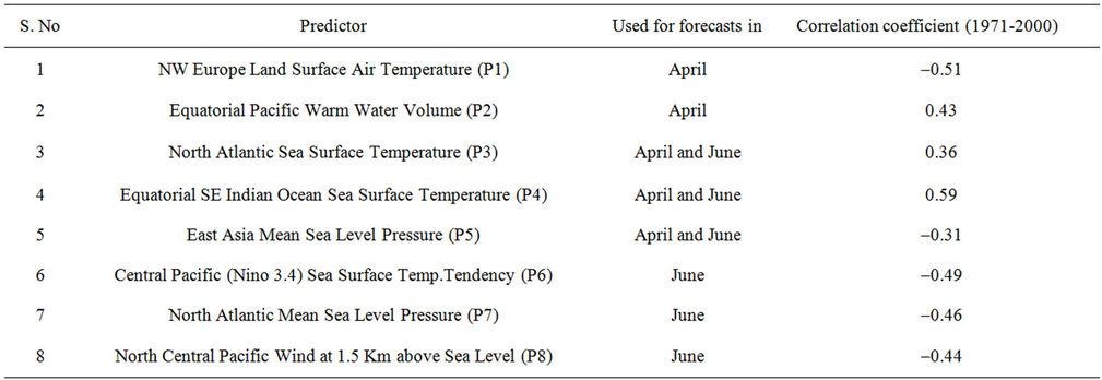
Table 2. Details of the 8 predictors used for the new ensemble forecast system.
possible to construct 31 (63) models. Using sliding fixed training window (of optimum period of 23 years, 1958- 1980) period, independent forecasts were prepared by all possible models for the period 1981-2008. For preparing ensemble average, a set of few best models from all possible MR models and another set of few best models from all possible PPR models are selected. The best models are selected in two steps. In the first step, all models (MR and PPR models separately) are ranked based on the objective criteria of likelihood function or generalized cross-validation (GCV) function computed for the period 1981-2007. In the second step, ensemble average of forecasts from the models ranked based on GCV values were computed by using first one model, first 2 models, and first 3 models and so on up to all the possible models in the rank list as the ensemble members. The ensemble average for each year of the independent period 1981-2007 was computed as the weighted average of the forecasts from the individual ensemble members. The weights used for this purpose was the C.C between the actual and model estimated ISMR values during the training period (of 23 years just prior to the year to be forecasted) adjusted for the model size. Mean of the two ensemble average forecasts (one from MR models and another from PPR models) was computed as the final forecast. Performance of the April and June forecast for the independent test period of 1981-2008 computed using the new ensemble method. The RMSE of the independent April & June forecasts for the period 1981-2008 was 5.9% of LPA and 5.6% of LPA respectively.
3. The New Three Stage Method Suggested
3.1. Parameters Considered as Potential Predictors
In the present study a three stage procedure is used. A set of 16 non-overlapping parameters (Table 3) from the set of 10 parameters (Table 1) used for the earlier 8 and 10 parameter model, which was used from 2003 to 2006 and also from the set of 8 parameters (Table 2) used for the new ensemble forecasting system introduced in 2007, is considered as the set of potential predictors for the model. The first 11 parameters (with data up to March) from these 16 parameters are used as the set of potential predictors for the models to be used for the first stage forecast of ISMR issued in April. The first 14 parameters (with data up to May) from these non-overlapping parameters are used as the set of potential predictors for the models to be used for the second stage forecast of ISMR issued in June. All the 16 parameters (with data up to June) are used for the final (third) stage forecast of ISMR issued in July.
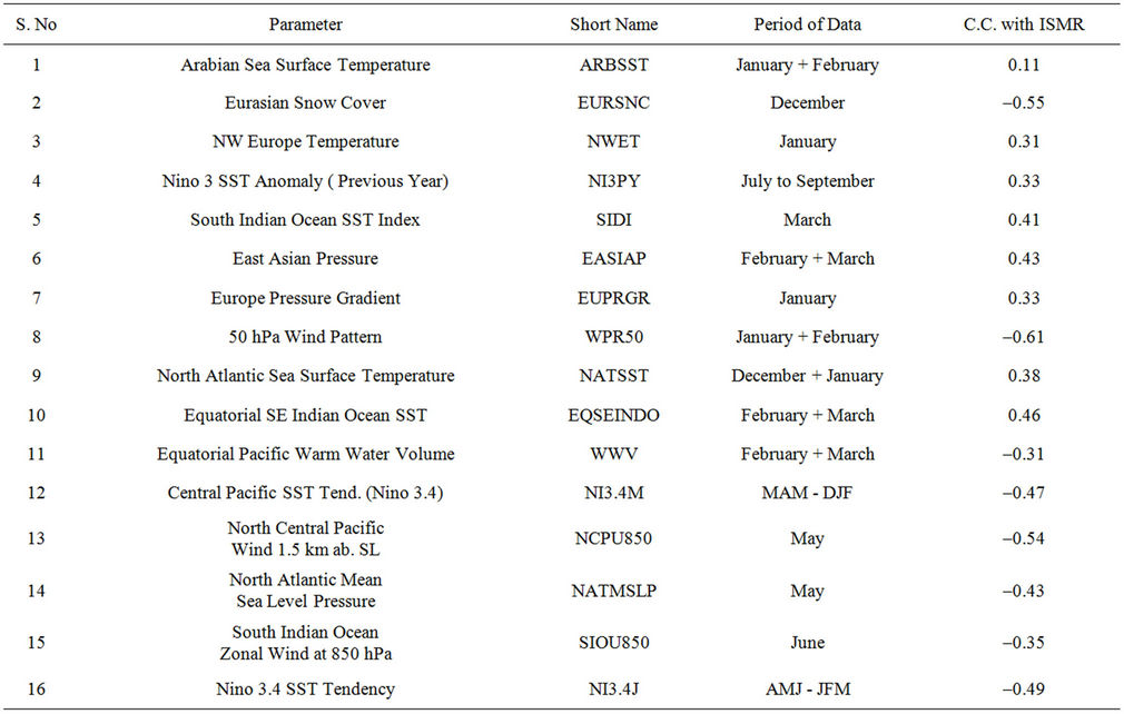
Table 3. List of 16 parameters used for developing new three stage forecast method.
3.2. Selecting the Most Pertinent Predictors
The most pertinent predictors that explain most of the variance are selected from the set of all potential predictors by using a stepwise selection procedure. In this procedure, selection of predictors is terminated if the new candidate predictor contributes less than a critical value, to the percentage of variance explained by the predictors already selected [10]. In order to have a significant percentage of variance explained by the predictors selected and to have less noise in the predictions, this critical value is taken as 0.5% [11,12]. If the variable recently selected is rejected in the selected variables while testing the significance then also the procedure is terminated.
Nine parameters (Table 4) including the June parameters are selected as the most pertinent predictors for the final(third) stage forecast of ISMR which is issued in July. These 9-parameters explain 83% of variance. 8-parameters (Table 5) including the May parameters are selected as the most pertinent predictors for the second stage forecast of ISMR which is issued in June. These 8 parameters explains 80% of variance. 6 parameters (Table 6) which are up to March are selected as the most pertinent predictors for the first stage forecast of ISMR which is issued in April. These 6 parameters explains 70% of variance.
8th parameter that is 50 hPa Wind Pattern (WPR50) in Table 3 is the fist parameter in the April and June models, but it is getting removed in the July models. Experiment is conducted for selecting the most pertinent predictors after removing it from the set of all potential predictors i.e. from Table 3. But the results gets deteriorated and the percentage of variance explained reduces to 79% and 67% for June and April models respectively and skill gets reduced for the validation data set as well. Hence it is the most important parameter for April and June models and models are developed and validated after including this parameter as explained in the above para.
3.3. Developing the Model Equations
The model equations are developed by using the most pertinent selected predictors for the first stage, second stage and third stage forecasts. These equations are developed using the linear regression and neural networks.
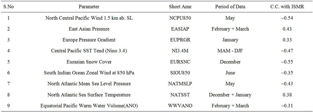
Table 4. List of parameters selected as predictors for third stage forecast in July.
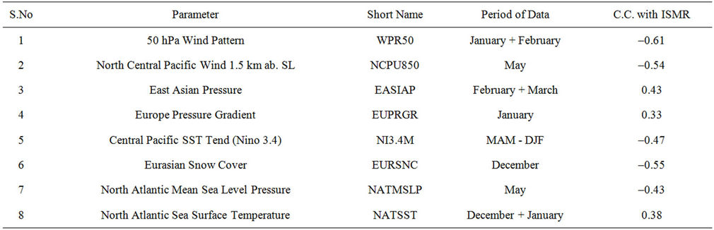
Table 5. List of parameters selected as predictors for second stage forecast in June.

Table 6. List of parameters selected as predictors for first stage forecast in April.
43 years of data from 1958 to 2000 for the predictors and predictands is used as the training set and next 11 years of data from 2001 to 2011 for the predictors and predictands is used as the validation set. Five types of equations using the five different predictands are developed for all the three stages of the forecast. These five different predictands are the following;
· Observed value of % anomaly of ISMR;
· Probability of more than normal ISMR that is percentage anomaly is greater than +4%;
· Probability of less than normal ISMR that is percentage anomaly is less than –4%;
· Probability of deficient ISMR that is percentage anomaly is less than –10%;
· Probability of excess ISMR that is percentage anomaly is more than 10%.
The probabilities for usual non-overlapping five categories can also be obtained from the above four probabilities as follows:

Here if the bigger class (e.g. less than normal) is having the less probability than the smaller class (e.g. deficient) then the smaller class is also given the same probability as the bigger class.
As the data available for developing the models is less, hence these over lapping probabilities are taken as predictands, so as to have good number of cases representing a particular class for the % anomaly of ISMR.
3.3.1. Linear Regression Equations
Simple linear regression equations of the Form (1) are obtained relating one predictand to the set of most pertinent selected predictors.
 (1)
(1)
where  are the multiple regression coefficients and
  are the values of the most pertinent selected predictors at the station. Here Y provides the predicted value of the predictand for a given set of predictors. These equations are developed by using the training data set of 43 years from 1958 to 2000 for all the four predictands as mentioned above and for all the three stages. The forecasts for predictands are obtained by putting the values of predictors by using the validation data set of 11 years from 2001 to 2011.
3.3.2. Neural Networks
Neural networks can have a massively parallel, layered structure with each layer consisting of several nodes called neurons. They provide a mapping from input vector xi, i = 1,2, ··· ,n, to the output vector yj, j = 1, 2, ··· ,m. Besides the input and output layers the network may also contain one or more hidden layers. Each neuron produces an output O = f(Z), where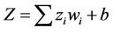 , zi (i = 1,2, ··· ,n) are the inputs to the given neuron, f(Z) is called the activation function and is usually taken to be the sigmoidal function
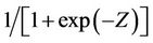 , wi are the weights associated with the network and b is the bias of the neuron. The weights wi and the bias b represent the parameters of the network which are to be determined by using the training data set of the pattern to be learned. Neural networks have the remarkable ability for pattern recognition [13]. It has been found that a two hidden layer network can learn most functions with compact domain. More details on neural networks and their applications can be found in the text books on neural networks such as [14,15].
The training algorithm used in the neural network for minimization of error is the conjugate gradients procedure complemented by simulated annealing to evade local minima. The conjugate gradients method is expected to be more efficient than the more commonly used back propogation algorithm and hence the network is expected to learn faster [14]. The simulated annealing method is necessary to escape from local minima which are usually present abundantly in the error function. The error measure was taken as the usual mean squared sum of errors.
In the present study one hidden layer with three neurons is used for developing the neural network equations for the predictands related to % anomaly of ISMR in order to match with the amount of data available. These equations are developed by using the training data set of 43 years from 1958 to 2000. The forecasts for predictands are obtained by putting the values of predictors by using the validation data set of 11 years from 2001 to 2011 as it was done in case of linear regression.
4. Evaluation of Forecast Skill
4.1. Skill Scores Used for Verification
Contingency tables are prepared for all the four type of predictands related to % anomaly of ISMR and all the three stages as mentioned in Section 3.3 and for both linear regression and neural networks.
The root mean square error, ratio score and Hanssen and Kuiper’s (HK) score are calculated for the forecasts for % anomaly of ISMR. The Brier score, ratio score and HK score are used for the forecasts for probability of more than normal, less than normal, deficient and excess conditions as mentioned in Section 3.3.
Brier score is defined as follows:

where {(fi ,xi), i = 1,2, ··· ,N} is data sample and  and
and  are the forecasted and observed probability values. The Brier score ranges from “0” to “1”.
Ratio score and HK score are calculated for YES/NO forecasts for all the stations. For a given 2 × 2 contingency table between forecast and observed rain situations, the HK score is defined as follows:

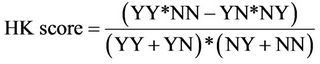

The value of HK score varies from “–1” to “+1”. If all forecasts are incorrect, that is YY = NN = 0 then HK score equals –1. If forecasts are prefect, that is YN = NY = 0, then the HK score equals +1.
4.2. Verification Results
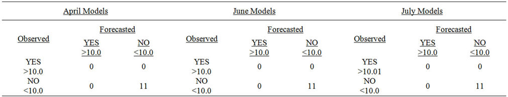
The Results for contingency tables for all the four type of predictands related to % anomaly of ISMR and all the three stages as mentioned in Section 3.3 and for both linear regression and neural networks, are given in the Tables 7-11. All the contingency tables for June and July models show at the most 1 to 3 non-matching cases out of 11 cases. July models show the high skill for all the five predictands. Although for the April models the non-matching cases are 4 out of 11 by using linear regression for probability of more than normal and deficient ISMR. This indicates the very high percentage of matching cases.
 (a)
(a)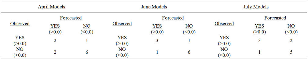 (b)
(b)
Table 7. 2 × 2 contingency table for % ANO for ISMR (YEARS: 2001 to 2009). (a) Linear Regression; (b) Neural Network.
 (a)
(a) (b)
(b)
Table 8. 2 × 2 contingency table for probability of more than normal (> 4% ANO) ISMR (YEARS: 2001 to 2009). (a) Linear regression; (b) Neural network.
 (a)
(a)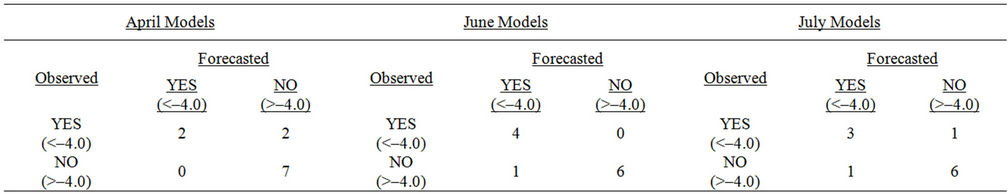 (b)
(b)
Table 9. 2× 2 contingency table for probability of less than normal (<–4% ANO) ISMR (YEARS: 2001 to 2009). (a) Linear regression; (b) Neural network.
The observed and forecasted values for all the five type of predictands related to % anomaly of ISMR and all the three stages as mentioned in section 3.3 and for both linear regression and neural networks, are plotted as from Figures 1(a) and (b) to Figures 3(c)-(e).
For the first stage that is April models, the predictions by using the neural network method had always been better than that by using the linear regression and the sign of predicted % anomaly of ISMR is same as that of observed for all 11 cases except for 1 case using linear egression and 2 by using neural networks, Figure 1(a). For probability of more than normal (>4% ANO) ISMR, the probability is not matching only for the year 2003, which is a positive ANO (+2%) case and for the year 2007 by using neural networks, Figure 1(b). For probability of less than normal (<–4% ANO) ISMR, the probability is not matching for two cases out of 11 cases by using neural networks, Figure 1(c). For probability of deficient conditions (<–10% ANO of ISMR), the probability is not matching for 3 cases out of 11 cases by using neural networks, Figure 1(d). For probability of excess conditions (>10% ANO of ISMR), the probability is matching for all the cases both for linear regression and neural networks, Figure 1(e).
 (a)
(a) (b)
(b)
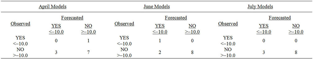
Table 10. 2 × 2 contingency table for probability of deficient (<–10% ANO) ISMR, (YEARS: 2001 to 2009). (a) Linear regression; (b) Neural network.
 (a)
(a) (b)
(b)
Table 11. 2 × 2 contingency table for probability of excess (> 10% ANO) ISMR (YEARS: 2001 to 2009). (a) Linear regression; (b) Neural network.
For the second stage that is June models, the predictions by using the neural network method had always been better than that by using the linear regression and the sign of predicted % anomaly of ISMR is same as that of observed for all 11 cases except for the years 2005 where the difference is very small that is from –1.00 to 3.74 and for the year 2011 where difference is very small that is from –0.24 to 1.73 by using neural networks, Figure 2(a). For probability of more than normal (>4% ANO) ISMR, the probability is not matching only for the year 2003, which is a positive ANO (+2%) case and for the year 2010 by using neural networks, Figure 2(b). For probability of less than normal (<–4% ANO) ISMR, the probability is not matching only for one case i.e. year 2006 by using neural networks and linear regression both, Figure 2(c). For probability of deficient conditions (<–10% ANO of ISMR), the probability is not matching for one case out of 11 cases by using neural networks, Figure 2(d). For probability of excess conditions (>10% ANO of ISMR), the probability is matching for all cases for linear regression and it is not matching for one case out of 11 cases by using neural networks, Figure 2(e).
For the third stage that is July models, the predictions by using the neural network method had always been
 (a)
(a) (b)
(b)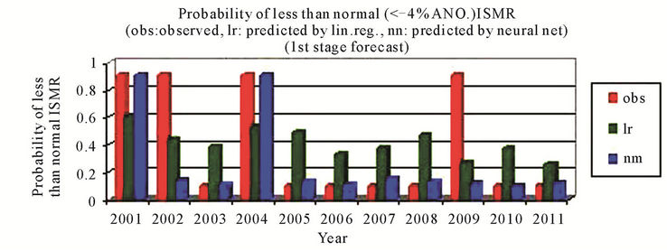 (c)
(c) (d)
(d) (e)
(e)
Figure 1. (a) & (b) observed and predicted (a) % anomaly of ISMR (b) probability of more than normal ISMR, as predicted by linear regression and neural network for the first stage forecast. (c)-(e) observed and predicted (c) probability of less than normal ISMR (d) probability of deficient ISMR (e) probability of excess ISMR, as predicted by linear regression and neural network for the first stage forecast.
 (a)
(a)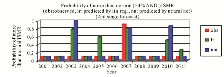 (b)
(b) (c)
(c)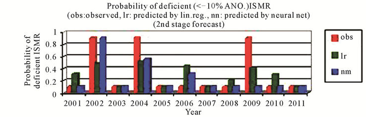 (d)
(d)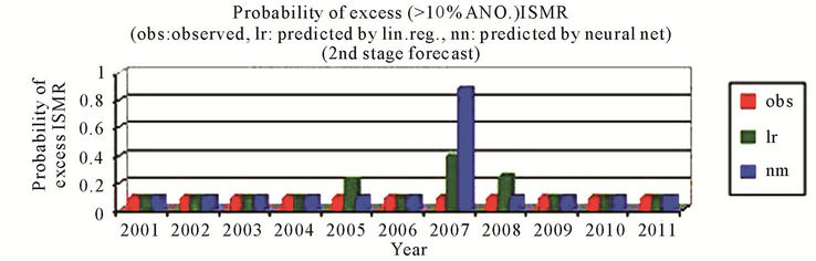 (e)
(e)
Figure 2. (a) & (b) observed and predicted (a) % anomaly of ISMR (b) probability of more than normal ISMR, as predicted by linear regression and neural network for the second stage forecast. (c)-(e) observed and predicted (c) probability of less than normal ISMR (d) probability of deficient ISMR (e) probability of excess ISMR, as predicted by linear regression and neural network for the second stage forecast.
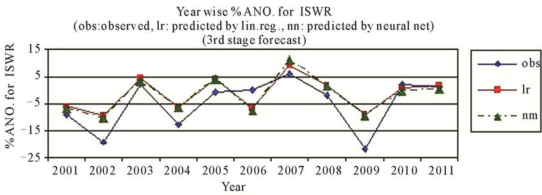
better than that by using the linear regression and the sign of predicted % anomaly of ISMR is same as that of observed for all cases except for the year 2010 where the difference is very small that is from –0.31 to 0.82 by using neural networks, Figure 3(a). For probability of more than normal (>4% ANO) ISMR, the probability is not matching only for the year 2003, which is a positive ANO (+2%) case and for the year 2005 by using neural networks, Figure 3(b). For probability of less than normal (<–4% ANO) ISMR, the probability is not matching only for the year 2006, which is a zero anomaly case by using neural networks, Figure 3(c). For probability of deficient conditions (<–10% ANO of ISMR), the probability is not matching only for the year 2001, which is a highly negative ANO (–9%) case and the year 2006 by using neural networks, Figure 3(d). For probability of excess conditions (>10% ANO of ISMR), the probability is matching for all the cases for linear regression and it is not matching for two cases out of 11 by using neural networks, Figure 3(e).
The root mean square error, ratio score and HK score for % anomaly of ISMR and Brier score, Ratio score and HK score for all the types of probability forecasts are given in Table 12.
For the first stage that is April models, rmse is 9.00, ratio score is 0.73 and HK score is 0.36 for the predictions of % anomaly of ISMR using neural networks and for probability predictions using neural networks brier score varies from 0.09 to 0.27, ratio score varies from 0.73 to 0.91 and HK score is up to 0.5, which is a moderate to high skill. For excess case brier score is 0.0 and ratio score is 1.00.
For the second stage that is June models, rmse is 5.69, ratio score is 0.82 and HK score is 0.61 for the predictions of % anomaly of ISMR using neural networks and for probability predictions using neural networks brier score varies from 0.09 to 0.16, ratio score varies 0.82 to 0.91 and HK score varies from 0.61 to 0.86, which is very high. For excess case brier score is 0.07 and ratio score is 0.91.
For the third stage that is July models, rmse is 6.19, ratio score is 0.73 and HK score is 0.46 for the predictions of % anomaly of ISMR using neural networks and for probability predictions using neural networks brier score varies from 0.11 to 0.18, ratio score is 0.82 and HK score varies from 0.61 to 0.80, which is also very high. For excess case brier score is 0.02 and ratio score is 1.00.
5. Conclusions
The contingency tables shows the high level matching cases in the validation set of 11 years (2001 to 2011) for all the three stages models except for April models in case of probability of more than normal ISMR and deficient
 (a)
(a)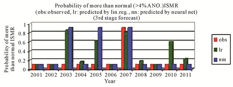 (b)
(b)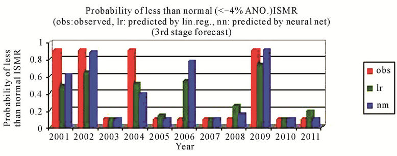 (c)
(c) (d)
(d)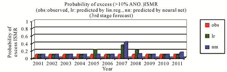 (e)
(e)
Figure 3. (a) & (b) observed and predicted (a) % anomaly of ISMR (b) probability of more than normal ISMR, as predicted by linear regression and neural network for the third stage forecast. (c)-(e) observed and predicted (c) probability of less than normal ISMR (d) probability of deficient ISMR (e) probability of excess ISMR, as predicted by linear regression and neural network for the third stage forecast.


Table 12. Skill scores of the forecasts for the % ANO for ISMR and related probabilities.
conditions. The neural networks are better as compared to linear regression in general although in some cases the linear regression is equally good.
As far as for the prediction for % anomaly of ISMR it is better for June models as compared to April models and July models are better for June models. The predictions by using neural networks are better as compared to that using by linear regression in general.
The predictions for the related probability predictands by using neural networks are also better as compared to those by using linear regression. The predictions for more than normal ISMR by using neural networks is having same skill for the models for all the three stages. The predictions for less than normal ISMR by using neural networks is highly improved for June and July models as compared to April models. Although the predictions for deficient conditions by using neural networks is also highly improved for June and July models as compared to April models, but July models are still better that June models.
The three stages (April, June and July) prediction system explained above is able to show high skill by using the robust technique like neural networks which was never attempted before. Moreover the skill of the forecast attained is found to be generally better as compared to the skill of the forecast obtained from the models attempted by other authors in the past [9]. The low value of rmse for the predicted % anomaly of ISMR and nearly prefect forecasts for the related probability predictands indicates that the procedure has the high potential to provide a prediction for ISMR, which would definitely improve the operational forecast of ISMR for the country.
6. Acknowledgements
I acknowledge the guidance and data provided by IMD, Pune in the present study. I express my sincere gratitude to Dr. Pankaj Jain from IIT, Kanpur for the basic routines used for neural network techniques in the present study. I also express my sincere thanks to G. R. Iyengar for his help in the overall write up of the research paper.
REFERENCES
- G. T. Walker, “A Further Study of Relationships with Indian Monsoon Rainfall-II,” Memoirs of the India Meteorological Department, Vol. 23, No. 8, 1914, pp. 123- 129.
- G. T. Walker, “Correlation in Seasonal Variations of Weather, VIII: A Preliminary Study of World Weather,” Memoirs of the India Meteorological Department, Vol. 24, No. 4, 1923, pp. 75-131.
- V. Thapliyal, “Stochastic Dynamic Model for Long Range Forecasting of Summer Monsoon Rainfall in Peninsular INDIA,” Mausam, Vol. 33, 1982, pp. 399-404.
- V. Gowariker, V. Thapliyal, R. P. Sarker, G. S. Mandal and D. R. Sikka, “Parametric and Power Regression Models: New Approach to Long Range Forecasting of Monsoon Rainfall in India,” Mausam, Vol. 40, 1989, pp. 115- 122.
- V. Gowariker, V. Thapliyal, S. M. Kulshrestha, G. S. Mandal, N. Sen Roy and D. R. Sikka, “A Power Regression Model for Long Range Forecast of Southwest Monsoon Rainfall over India,” Mausam, Vol. 42, 1991, pp. 125-130.
- M. Rajeevan, D. S. Pai, S. K. Dikshit and R. R. Kelker, “IMD’s New Operational Models for Long Range Forecast of South-West Monsoon Rainfall over India and Their Verification for 2003,” Current Science, Vol. 86, No. 3, 2004, pp. 422-431.
- D. S. Wilks, “Statistical Methods in Atmospheric Sciences,” Academic Press, Waltham, 1995.
- M. Rajeevan, P. Guhathakurta and V. Thapliyal, “New Models for Long Range Forecasts of Summer Monsoon Rainfall over Northwest and Peninsular India,” Meteorology and Atmospheric Physics, Vol. 73, No. 3-4, 2000, pp. 211-225. doi:10.1007/s007030050074
- M. Rajeevan, D. S. Pai, R. A. Kumar and B. Lal, “New Statistical Models for Long Range Forecasting of SouthWest Monsoon Rainfall over India,” Climate Dynamics, Vol. 28, No. 7-8, 2007, pp. 813-828. doi:10.1007/s00382-006-0197-6
- R. G. Tapp, F. Woodcock and G. A. Mills, “Application of MOS to Precipitation Prediction in Australia,” Monthly Weather Review, Vol. 114, No. 1, 1986, pp. 50‑61. doi:10.1175/1520-0493(1986)114<0050:TAOMOS>2.0.CO;2
- A. Kumar and P. Maini, “An Experimental Medium Range Local Weather Forecast Based upon Global Circulation Model at NCMRWF, TROPMAT 1993,” Indian Meteorological Society, New Delhi, 1993, pp. 48‑55.
- A. Kumar and P. Maini, “Statistical Interpretation of General Circulation Model: A Prospect for Automation of Medium Range Local Weather Forecast in India,” Mausam, Vol. 47, No. 3, 1996, pp. 227‑234.
- P. Jain, A. Kumar, P. Maini and S. V. Singh, “Short Range SW Monsoon Rainfall Forecasting over India Using Neural Networks,” Mausam, Vol. 53, No. 2, 2002, pp. 225-232.
- T. Masters, “Practical Neural Network Recipes in C++,” Academic Press, Waltham, 1993, p. 493.
- B. Muller and J. Reinhardt, “Neural Networks: An Introduction. The Physics of Neural Networks Series,” Springer-Verlag, Berlin, 1991, 266 pages.
NOTES
*Corresponding author.