Journal of Sensor Technology
Vol. 2 No. 2 (2012) , Article ID: 19686 , 7 pages DOI:10.4236/jst.2012.22013
Application of the HES in Angular Analysis
1Department of Intelligent Mechanical Engineering, Faculty of Engineering, Fukuoka Institute of Technology, Fukuoka, Japan
2Faculty of Engineering, Ramkhamhaeng University, Bangkok, Thailand
Email: kswitsar@kmitl.ac.th
Received April 5, 2012; revised May 1, 2012; accepted May 11, 2012
Keywords: Angle; Axis; Decline; Degree; Electromagnetic Field; Helmholtz Coil; HES; Shaft
ABSTRACT
This study presents an analysis of the relationship of angles and trigonometric functions by applying Hall Effect Sensor (HES). Electromagnetic density of 4.624 mT can be generated from the Helmholtz coil. Angle of shaft which was installed at the center of the Helmholtz coil perpendicularly to horizontal plane was considered as reference and can be rotated. In this study, an experiment for measuring the angle of shaft declination on X-axis was carried on. Ranges of measurement were related to the angle resolution between –15 to 15 degree with 1 step degree interval from perpendicular angle (Y-axis). Analysis of the relationship between shaft declination and electromagnetic field was performed using HES device which was installed on the top of shaft and perpendicularly to reference electromagnetic field [1,2]. The angle declining from the origin which was normal to magnetic field can be determined by measuring the relationship between Hall voltage and magnetic field. Normally, electromagnetic field is nonuniform and varied by point in Helmholtz coil radius. Shaft angles on X-axis were measured for assessing the repeatability of system developed. Five values of results were measured repeatedly at the same input. It can be observed that the system developed can provide the results with the best accuracy and reliability of 95%.
1. Introduction
Angular displacement is one of important variables in industrial processes such as industrial machine alignment and installation and also in civil engineering studies. This study presents the alternative methodology to examine the angular displacement of shaft using magnetic field method. Hall Effect Sensor (HES) was used as a sensor for analyzing the relationship of trigonometric functions in terms of angle and remaining length of the measured triangle. In this study, the declined angle of shaft on X-axis was assessed despite measurement and analysis of angular position (ranging from 0 to 360 degree) [3-5]. Output voltages from the HES were also available for real time collection via PC which can be then used for further analysis.
2. Fundamental Method
2.1. Design of the Helmholtz Coil
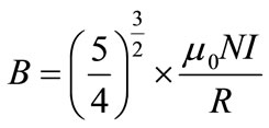
Two Helmholtz coils, serial wires, were used in this study. These coils were mounted parallelly with the gap equal to coil radius. Then, electromagnetic field generated at the center of Helmholtz coil was found to be stable and magnetic flux was distributed from the center of coil [6]. The density of the electromagnetic field was proportional to the number of wire turns and induced by external constant current. The relationships of current supplied constantly to Helmholtz coil and density of electromagnetic field can be expressed in Equation (1).
 (1)
(1)
where B is density of magnetic field (Tesla);
m0 is magnetic permeability (1.26 × 10⁻⁶ Tm/A);
N is number of turn of each sub-coil (Turn);
I is current through each coil (A);
R is coil radius or distance between coils (m).
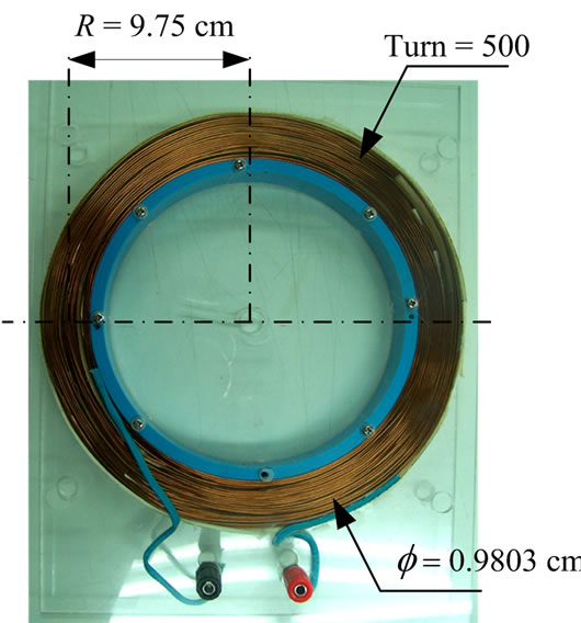
Design principle of Helmholtz coil in this study was considered the ratio of wire-turn thickness and radius of Helmholtz coil by 1:5. Therefore, the thickness (t) was 2 cm with the Radius (R) of 9.75 cm from 500 turns of 0.9803 mm copper wire (AWG 19 standard) as shown in Figure 1. Figures 1(a) and (b) illustrate an electromagnetic field generator and an alignment of Helmholtz coil, respectively.
2.2. Relationship of Trigonometric Function and Electromagnetic Field
The relationship of electromagnetic field density in any point within Helmholtz coil radius and declined angle of
 (a)
(a)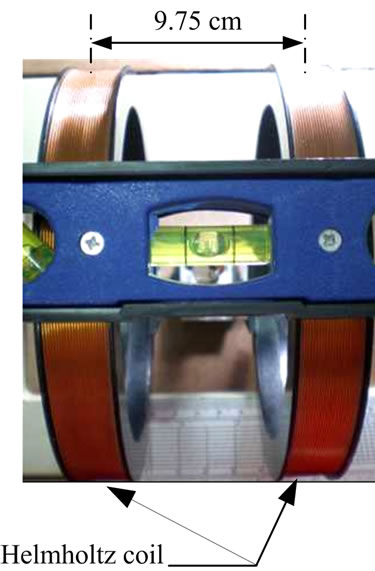 (b)
(b)
Figure 1. Structure of the generator for generate electromagnetic field constant: (a) Electromagnetic field generator; (b) Side view of the Helmholtz coil alignment.
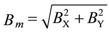
shaft can be determined by the current flowing into the coil in one cycle as shown in Figure 2. Also, an analysis of phase movement (Bm) can be expressed by Equation (2).
 (2)
(2)
where Bm is movement of phases;
B0 is center of the magnetic field;
BX is phases movement direction X-axis;
BY is phases movement direction Y-axis;
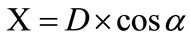
An analysis of angle (q) due to shaft declination on X-axis compared to the center of Helmholtz coil was performed as shown in Figure 3. The distribution properties of magnetic field density at a given point within Helmholtz coil radius can be estimated by Equations (3), (4) and (5), respectively.
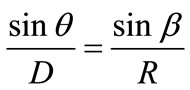 (3)
(3)
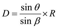 (4)
(4)
 (5)
(5)
where q is decline angle of shaft;
R is length of shaft;
D is distance of the end of shaft from the center of the Helmholtz coil;
X is distance of shaft from center of the Helmholtz coil direction X-axis;
b is angular of the triangle base.
2.3. Principle of HES
HES is a small passive transducer (non-contact sensor) which is applicable in several purposes. The output voltage can be generated when the constant current transmitting through a semiconductor namely Hall generator is diverted [7] as shown in Figure 4.
The magnetic density (B) generated by sensing module can be analyzed by Lorenzt force (F) of the magnetic field on an electron (q) when changing the relative angle
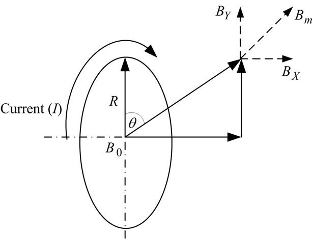
Figure 2. The relationship of electromagnetic field and current flowing into the coil.
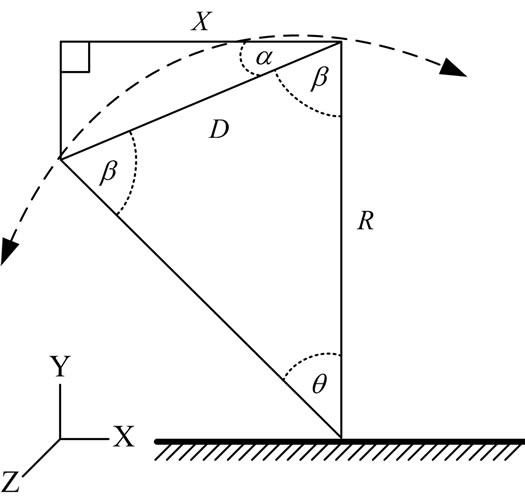
Figure 3. Relationship of the trigonometric function compared with the center of Helmholtz coil.
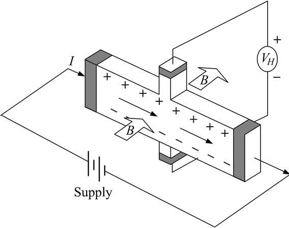
Figure 4. Direction of current transmitting through Hall generator.
 as given in Equation (6). v is the velocity of electron due to electric field.
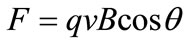 (6)
(6)
Therefore, we have using the HES No. A1301 (UA suffix) type 3 pin SIP (Continuous-Time Ratio metric Linear HES ICs) as a sensor and analysis in this study.
3. Structure of System Developed
The system developed for analysis of shaft declination consists of two Helmholtz coils with radius (R) of 9.75 cm, placed at the structure of 8 mm-thick acrylic plates with the shaft length of 30 cm. The reference scale perpendicularly placed on the 5 cm-thick acrylic rod for adjusting the declined angle in experiment as shown in Figure 5 and the reference scale used for measuring an accuracy of angular declination in each degree of shaft [8].
To detect the electromagnetic field density in any position within Helmholtz coil radius, the sensor namely HES was placed at the centre between two Helmholtz coils as shown in Figure 6. Variability of the output voltage from the HES was then considered. There is a relation between a density of electromagnetic field generated by applying 1 Amp current into the Helmholtz coil and the output voltage from the HES. Figure 7 shows the constant current power supply and the Data Acquisition (DAQ) which was connected to a computer for collecting and analyzing data via PC-Based DAQ System.
4. Electromagnetic Field Generation
In this study, wave form of electromagnetic field was analyzed from the gap of two Helmholtz coils using COMSOL software simulation. The gap of two coils was fixed by 0.8 R space, R space and 1.2 R of coil space. The results obtained from simulation are as shown in Figures 8-10 where Y-axis is the density of the electromagnetic field and X-axis is declination of shaft within Helmholtz coil radius.
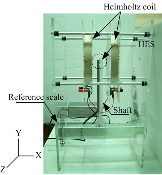
Figure 5. Side view of the system developed.
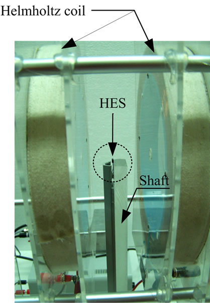
Figure 6. HES position at the centre between two Helmholtz coils.
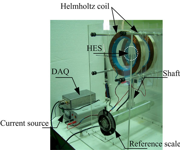
Figure 7. Constant current power supply for Helmholtz coil.
The results from COMSOL simulation at any distance position of the Helmholtz coil under the same condition can be indicated that the coils mounted parallelly at 0.8 R of space would exhibit in the large graph as well as the slope and the width would be greater than Dead band. In
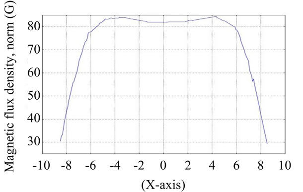
Figure 8. The space of two coils was 0.8 R.
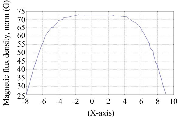
Figure 9. The space of two coils was R.
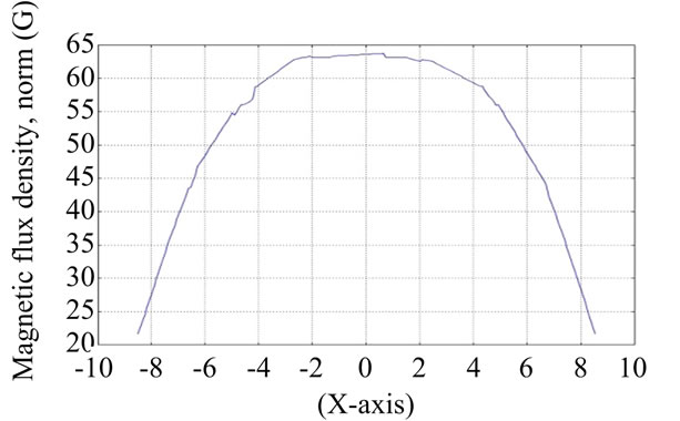
Figure 10. The space of two coils was 1.2 R.
case of 1.2 R space of coils, the graph would be small and the slope would be declined less than Dead band. Considering R space of coils, it can be noted that the relationship of angle and electromagnetic field is well balance. Therefore, the space of the Helmholtz coils in this study was fixed at R.
The density of the electromagnetic field generated by the Helmholtz coil can be measured using Tesla meter (PHYWE) with the resolution of 1 mT at the reference position (0 degree). A probe was installed at the center of Helmholtz coil and the constant current of 1 Amp was provided for generating electromagnetic field with the density of 4.624 mT (from calculation). From experiment, the density of electromagnetic field measured at the center of the Helmholtz coil was 5 mT after compensating an error. The discrepancy from analysis was 0.376 mT (7.52%) that would be caused by the resolution of the Tesla meter used as shown in Figure 11.
5. Experimental and Analysis
Analysis of shaft declination angle was based on trigonometric function. The system developed was designed the shaft to be declined on X-axis in both (+) and (–) directions ranging from 0 to ±15 degree (normal to Y-axis) with 1 degree resolution per step as shown in Figure 12. To analysis the density of the electromagnetic field at any position within the Helmholtz coil radius, the shaft was angularly moved on the X-axis starting from the reference point (0 degree) as shown in Figure 13. The measured results were presented in output voltage which varied by the current flowing through the HES and depending on electromagnetic field density. However, the output voltage of the HES was also dependent on the density and direction of magnetic field which varied from 0 degree (2.77 Volt) to ± 15 degree (2.65 Volt).
Experimental results can be used for analysis of the relationship of output voltage from HES and electromagnetic field density within the Helmholtz coil radius on X-axis as showing the graph in Figure 14. The results agree well to the results from calculation using COMSOL software simulation. The gap between two coils of Helmholtz coils was equal to R. The relationship can be expressed by the variation of output voltage through a fourth degree polynomial as given in Equation (7).
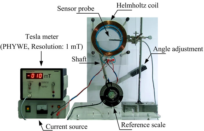
Figure 11. Reference point of the HES.
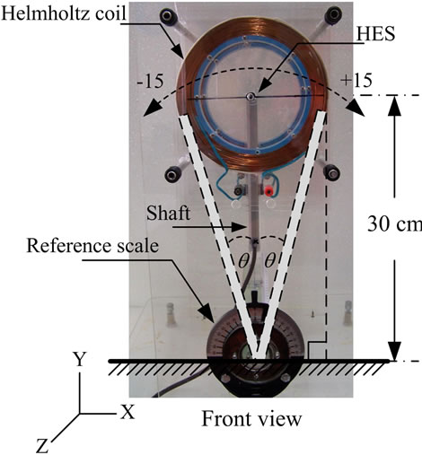
Figure 12. Shaft declination on X-axis.
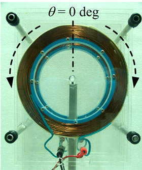
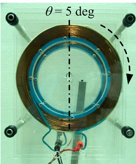
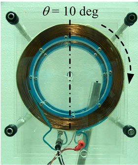

Figure 13. Shaft declination by step varying from 0 to +15 degree.
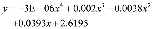 (7)
(7)
where y is output voltage from the HES (Volt) x is ranges of measurement (degree)
Considering the angle of shaft declination by repeatedly measuring 5 values and then comparing to actual values, it can be noted that the measured declination angle exhibited the results with high accuracy, precision and reliability at every angle in the range between 0 to ±15 degree, except the range of 2 to –3 degree as shown in Figure 15. It was due to low difference of the output voltage from the HES which could not be distinguished; this range was therefore Dead band of output signal which agreed well to calculation results using COMSOL software simulation.
In experimental study, accuracy, precision, and reliability were analyzed by considering the Average Value (AVG), Standard Deviation (STD) and Experimental Uncertainty (Uc) [9]. In analysis of the HES output voltage,
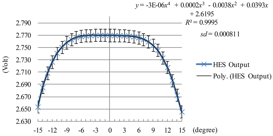
Figure 14. Relationship of output voltage from the HES and electromagnetic field density.
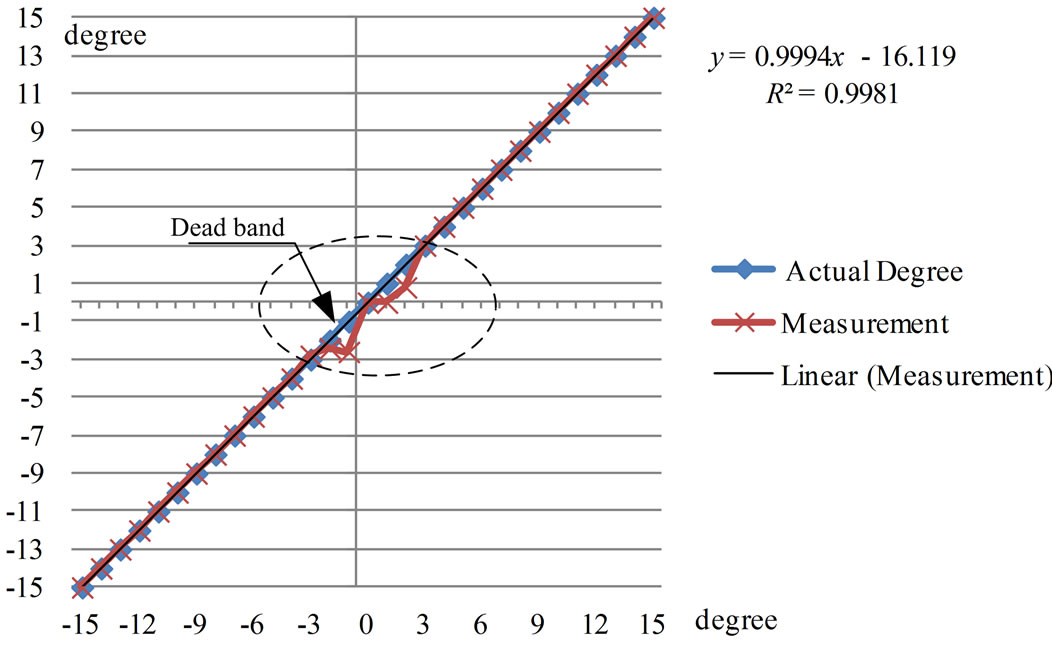
Figure 15. Dead band in the range of 2 to –3 degree.
it can be observed that the declination of the shaft at any position within the Helmholtz coil radius would exhibit the best accuracy and reliability of 95%. The maximum error was at –3 degree or equal to 0.734847 as shown in Table 1.
Conclusively, the output voltage of the HES can be used for analyzing the angles of sine, cosine, and tangent of the trigonometric functions as well as the length of triangle. The results from experiment and also the range of Dead band agreed well to those from calculation. Angular positions of shaft with declination on X-axis are as shown in Figures 16-20.
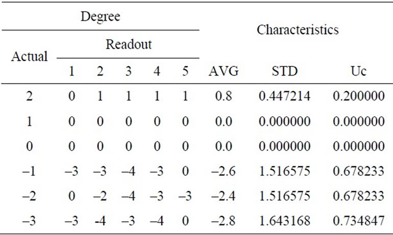
Table 1. Error within the range of 2 to –3 degree.
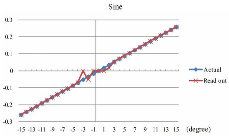
Figure 16. Comparison of sine from experiment and calculation.
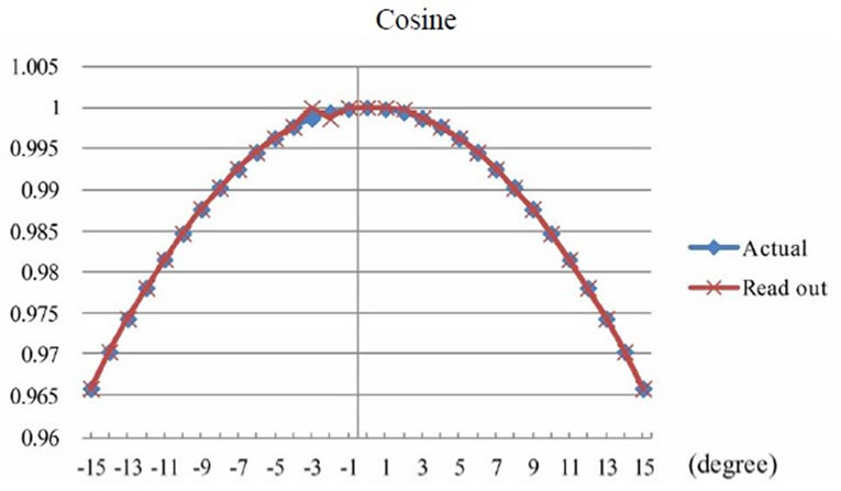
Figure 17. Comparison of cosine from experiment and calculation.
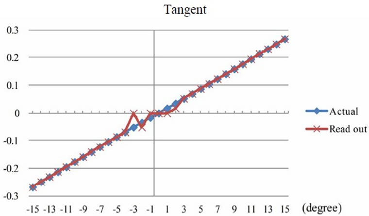
Figure 18. Comparison of tangent from experiment and calculation.
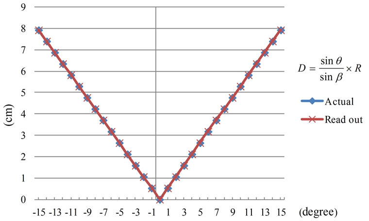
Figure 19. Comparison of D distance from experiment and calculation.
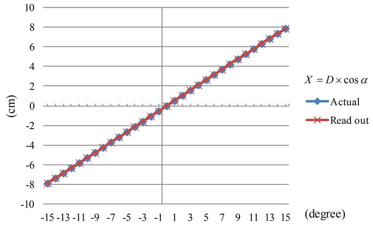
Figure 20. Comparison of X distance from experiment and calculation.
6. Conclusion
From experimental study of sensor angular position by analyzing the HES output voltage, it can be observed the relationship of Hall voltage and the density of electromagnetic field within the Helmholtz coil radius. Moreover, the experimental results from the HES output voltage were varied by the density and direction of electromagnetic field generated by the Helmholtz coil. Dead band from testing was varied between 2 to –3 degrees according to the theory. However, Dead band would be dependent on magnetic field generated whether from Helmholtz coil or permanent magnet. To reduce the effect of Dead Band, permanent magnet and ADC with 16-bit resolution are recommended to adopt. In statistical analysis, the results from the system developed were found to provide high accuracy and reliability throughout experimental range (95%). The maximum uncertainty was 0.734847 at –3 degree.
REFERENCES
- C. Chaiyachit, S. Satthamsakul, W. Sriratana and T. Suesut, “Hall Effect Sensor for Measuring Metal Particles in Lubricant,” International Multiconference of Engineers and Computer Scientists, Hong Kong, 14-16 March 2012, pp. 894-897.
- W. Sriratana, K. Nakmee and L. Tanachaikhan, “Subsidence Monitoring System for Industrial Machines Based on Magnetic Field Method,” International Conference on Control, Automation and Systems, Seoul, 27-30 October 2010, pp. 346-349.
- V. Hiligsmann and P. Riendeau, “Monolithic 360 Degrees Rotary Position Sensor IC,” IEEE Sensors Conference, Vienna, 24-27 October 2004, pp. 1137-1142.
- B. Lequesne and T. Schroeder, “High-Accuracy Magnetic Position Encoder Concept,” IEEE Transactions on Industry Applications, Vol. 35, No. 3, 1999, pp. 568-576. doi:10.1109/28.767003
- Y. Y. Lee, R. H. Wu and S. T. Xu, “Applications of Linear Hall-Effect Sensors on Angular Measurement,” 2011 IEEE International Conference on Control Applications (CCA), Denver, 28-30 September 2011, pp. 479-482. doi:10.1109/CCA.2011.6044465
- G. Arfken, “Mathematical Methods for Physicists,” Academic Press, Orlando, 1985.
- E. Ramsden, “Hall-Effect Sensor: Theory and Applications,” Elsevier, Burlington, 2006.
- L. Tanachaikhan, N. Tammarugwattana, W. Sriratana and P. Klongratog, “Declined Angle Analysis of Shaft Using Magnetic Field Measurement,” ICROS-SICE International Joint Conference 2009, Fukuoka, 18-21 August 2009, pp. 1846-1849.
- United Kingdom Accreditation Service, “The Expression of Uncertainty and Confidence in Measurement,” United Kingdom Accreditation Service, London, 1997.