Advances in Chemical Engineering and Science
Vol.04 No.04(2014), Article ID:50302,23 pages
10.4236/aces.2014.44047
Design of a Simulator for Enhanced Oil Recovery Process Using a Nigerian Reservoir as a Case Study
Kamilu Folorunsho Oyedeko1*, Alfred Akpoveta Susu2
1Department of Chemical & Polymer Engineering, Lagos State University, Epe, Lagos, Nigeria
2Department of Chemical Engineering, University of Lagos, Lagos, Nigeria
Email: *kfkoyedeko@yahoo.com, alfredasusu222@hotmail.com
Copyright © 2014 by authors and Scientific Research Publishing Inc.
This work is licensed under the Creative Commons Attribution International License (CC BY).
http://creativecommons.org/licenses/by/4.0/

![]()

Received 21 July 2014; revised 18 August 2014; accepted 28 August 2014
ABSTRACT
This study involves the applications of different numerical techniques in a more general way to the design of a simulator for an enhanced oil recovery process with surfactant assisted water flooding. The data from a hypothetical oil well and a Nigerian oil well were used for the validation of the simulator. The process is represented by a system of nonlinear partial differential equations: the continuity equation for the transport of the components and Darcy’s equation for the phase flow. The orthogonal collocation, finite difference and coherence theory techniques were used in solving the equations that characterized the multidimensional, multiphase and multicomponent flow problem. Matlab computer programs were used for the numerical solution of the model equ- ations. The predicted simulator, obtained from the resulting numerical exercise confers uncondi- tional stability and more insight into the physical reservoir description. The results of the ortho- gonal collocation solution were compared with those of finite difference and coherence solutions. The results indicate that the concentration of surfactants for orthogonal collocation show more features than the predictions of the coherence solution and the finite difference, offering more opportunities for further understanding of the physical nature of the complex problem. We have found out that the partition of the three components between the two-phases determines other physical property data and hence the oil recovery. The oil recovery for the Nigerian oil reservoir is higher than the recovery predicted for the hypothetical crude. The displacement mechanism for the multicomponent and multiphase system is stable in the Nigerian oil reservoir due to the mod- erate value of the oil/water viscosity instead of the hypothetical reservoir with high value of oil/water ratio.
Keywords:
Enhanced oil Recovery, Simulator Design, Multidimensional, Multicomponent and Multiphase System, Surfactant Assisted Flooding, Orthogonal Collocation, Finite Difference, Coherence Theory, Hypothetical Reservoir, Nigerian Reservoir

1. Introduction
The world economy today can be characterized as a crude oil economy. So far, there has not been a single energy source that has broadly been integrated to replace crude oil in the provision of electricity (light and heat) and transportation (land, air and sea). It is very important to at least, maintain or indeed, increase the current production levels of crude oil. These objectives can be accomplished by further investing in exploration and production of new fields or optimizing production from existing fields. Bringing new fields online can be expensive, while recovery from existing fields by conventional methods (i.e. primary and secondary recovery) will not fully provide the necessary relief for global oil demand.
On an average, only about a third of the original oil in place can be recovered by primary and secondary recovery processes. The rest of the oil is trapped in reservoir pores due to surface and interfacial forces. This trapped oil can be recovered by reducing the capillary forces that prevent oil from flowing within the pores of reservoir rock and into the well bores. Due to high oil prices and declining production in many regions around the globe, the application of advance technologies called “Enhanced Oil Recovery” (EOR) has become very attractive for exploration and production of the trapped oil. This technology requires the injection of a fluid or fluids or materials into a reservoir to supplement the natural energy present in a reservoir, where the injected fluids interact with the reservoir rock/oil/brine system to create favourable conditions for maximum oil recovery. Surfactants are injected to decrease the interfacial tension between oil and water in order to mobilize the oil trapped after secondary recovery by water flooding.
In a surfactant flood, a multi-component multiphase system is involved. The theory of multi-component, multiphase flow has been presented by several authors. The surfactant flooding is a form of chemical flooding and is represented by a system of nonlinear partial differential equations: the continuity equation for the transport of the components and Darcy’s equation for the phase flow. The system of equations is completed by the equations representing physical properties of the fluids and the rock. From a physico-chemical point of view, there are three components—water, petroleum and chemical. They are in fact, pseudo-components, since each one consists of several pure components. Petroleum is a complex mixture of many hydrocarbons. Water is actually brine, and contains dissolved salts. Finally, the chemical contains different kinds of surfactants. These components are distributed between two phases—the oleic phase and the aqueous phase. The chemical has an amphiphilic character. It makes the oleic phase at least partially miscible with water or the aqueous phase, partially miscible with petroleum.
Interfacial tension depends on the surfactant partition between the two phases. Residual phase saturation decreases as interfacial tension decreases. Relative permeability parameters depend on residual phase saturations. In addition, phase viscosities are functions of the volume fraction of the components in each fluid phase. Therefore, the success or failure of surfactant flooding processes depends on phase behaviour. Phase behaviour influences all other physical properties, and each of them, in turn influences oil recovery.
The different mathematical techniques used here, orthogonal collocation method, finite difference and coherence theory methods, are utilized for identification of particular physical behaviour. Besides, they may enable the understanding of the involved propagation phenomena in terms of cause and effects. More so, the techniques will in particular be utilized to predict what happens in EOR process and show how the complexity of the problem can be reduced by intensive calculation.
Systems of coupled, first-order, nonlinear hyperbolic partial differential equations (p.d.e.s) govern the transient evolution of a chemical flooding process for enhanced oil recovery. The method of characteristics (MOC) provides a way in which such systems of hyperbolic p.d.e.s can be solved by converting them to an equivalent system of ordinary differential equations. In fact, the MOC provides a similar framework for algorithm development to the coherence approach which is one of the numerical methods adopted here. In some cases, the characteristic solution has been used to track the flood-front in two-dimensional reservoir problems [1] . While the approach proposed by Ewing et al. [2] , combines the characteristic method with a finite element approach, Zheng [3] used the MOC and an adjustable number of moving particles to track three-dimensional solute fronts in groundwater systems by adjusting the number of particles served to maintain an accurate material balance and save computational time. This front-tracking approach has been used in the present work to trace the movement of coherent waves, of both the diffuse and shock variety.
The concept of coherence was extended to general EOR processes [4] [5] , including alkaline flooding [6] , convectional surfactant flooding [7] the effects of cation-exchange on surfactant-polymer flooding [8] [9] and miscible gas injection processes such as CO2 flooding (Orr et al., 1995; Wang and Orr, 1997). Refinements to the theory also allowed for equilibrium reaction to occur, such as precipitation-dissolution [10] [11] and micelle formation [12] . Helset and Lake [13] have used simple wave theory (essentially identical to coherence theory) to study the one dimensional, three phase secondary migration of hydrocarbons from a source rock into possible reservoirs. Most recently, the theory of coherence has been applied successfully to the analysis of the transport of volatile compounds in porous media in the presence of a trapped gas phase [14] .
At the simple level, the results of simulation using the principle of coherence are analogous to the Buckley-Leverett theory for water flooding, the latter being evident in the work of Patton et al. [15] for polymer flooding, Fayers and Perrine [16] for dilute surfactant flooding, Claridge and Bondor [17] for carbonated water flooding and Larson [18] and Hirasaki [7] for miscible and immiscible surfactant flooding, respectively. Pope, et al. [19] for isothermal, multiphase, multicomponent fluid Flow in permeable media. Hankins and Harwell [20] . Case studies for the feasibility of sweep improvement in surfactant-assisted water flooding. Other works on EOR researches include the work of Siggel, et al. [21] for a new class of viscoelastic surfactants for EOR, Xu and Lu [22] for microbially enhanced oil recovery at simulated reservoir conditions by use of engineered bacteria, Andrew Leach and Mason [23] for co-optimization of enhanced oil recovery and carbon sequestration, Harwell [24] for development of improved surfactants and EOR methods for small operators and many others.
So, in this work, we apply the different numerical techniques, orthogonal collocation, finite difference and coherence theory method, in solving the basic model transport equations characterizing the design of the simulator. As far as the authors are aware, this is the first time that the orthogonal collocation method is being applied to simulator design. The approach is multidimensional and involves at least three independent variables with the introduction of the concept of partial coherence so that the various composition path spaces required for mapping the composition routes of the system are at most two dimensional.
2. Methodology
In this work, we considered solving multidimensional, multicomponent, multiphase flow problems associated with enhanced oil recovery process in petroleum engineering. The process of interest involves the injection of surfactant of different concentrations and pore volume to displace oil from the reservoir.
The methodology indicates the steps utilized in executing the project using the developed mathematical models to describe the physics of reservoir depletion and fluid flow in which one of the main aims is the determination of the areal distribution of fluids in the reservoir resulting from a flood. The system is for two or three dimensions, two fluid phases (aqueous, oleic) and one adsorbent phase, four components (oil, water, surfactants 1 and 2).
The reservoir may be divided into discrete grid blocks which may each be characterized by having different reservoir properties. The flow of fluids from a block is governed by the principle of mass conservation coupled with Darcy’s law. The simultaneous flow of oil, gas, and water, in three dimensions and the effects of natural water influx, fluid compressibility, mass transfer between gas and liquid phases and the variation of such parameters as porosity and permeability, as functions of pressure are then modelled.
The model is developed from the basic law of conservation of mass [25] . The developed partial differential equation is converted to ordinary differential equation using coherent, finite difference and orthogonal collocation methods.
The finite difference method is a technique that converts partial differential equations into a system of linear equations. There are essentially three finite difference techniques. The explicit, finite difference method converts the partial differential equations into an algebraic equation which can be solved by stepping forward (forward difference), backward (backward difference) or centrally (central difference).
The orthogonal collocation method converts partial differential equations into a system of ordinary differential equations using the lagrangian polynomial method. The set of ordinary differential equations generated is then solved with appropriate numerical technique, in this work, by the explicit Runge Kutta method. The motivation for this explicit method is the simplicity and computation and efficiency and possibility of reducing truncation error over the required for other methods.
The coherent theory method combines the forward finite difference method with Runge Kutta technique to solve partial differential equations.
The rock and fluid properties such as density, porosity, viscosity, oil and water etc, and other parameters are listed in Tables 1-4. Table 1 is the Reservoir characteristics from the work by Hankins and Harwell [25] . Table 2 is the Reservoir Characteristics used for the Simulation work by Oyedeko [26] . Parameter values used in Trogus adsorption model for verification runs is shown in Table 3 while Table 4 is the Additional Reservoir Parameters for the coherence work by Hankins and Harwell [25] .
The model encompasses two fluid phases (aqueous and oleic), one adsorbent phase (rock), and four components (oil, water, surfactants 1 and 2). The oil is displaced by water flooding. In-situ interaction of surfactant slugs may occur, with consequent phase separation and local permeability reduction. The model accommodates two (or three) physical dimensions, and an arbitrary, nonisotropic description of absolute permeability variation and porosity.
For most of the simulated cases in the work of Harkins and Harwell [25] , the reservoir consisted of a rectangular composite of horizontal oil bearing strata, sandwiched above and below by two impervious rocks. Oil is produced from the reservoir by means of water injection at one end and a production well at the other. Data for the hypothetical reservoir simulated in Hankins and Harwell [25] are given in Table 6 and the model developed is given as:

Table 1. Reservoir characteristics from the work of Hankins and Harwell [25] .
Table 2. Reservoir characteristics used for the simulation work by Oyedeko [26] .
Table 3. Parameter values used in Trogus adsorption model for verification runs.
Table 4. Additional reservoir parameters for the coherence work by Hankin and Harwell [25] .
![]() (1)
(1)
The term ![]() represents the rate of loss of surfactant due to precipitation: for a one-to-one reaction stoichiometry,
represents the rate of loss of surfactant due to precipitation: for a one-to-one reaction stoichiometry,![]() . Since reaction occurs instantaneously at a sharp interface, this term may be ignored away from the singular region of the interface.
. Since reaction occurs instantaneously at a sharp interface, this term may be ignored away from the singular region of the interface.
It is possible to approximate the adsorption isotherm of a pure surfactant on a mineral oxide by use of a simple model. At low concentration the adsorption obeys Henry’s law, while above the critical micelle concentration (CMC) the total adsorption remains constant. The Trogus adsorption model [12] [27] is used in this work.
2.1. Application of Coherence Theory to the Solution of Model Equations
The material balance equations, Equation (1) (in the absence of![]() ), are first order, homogeneous, nonlinear hyperbolic equations. Their solution will be attempted by means of the theory of coherence. The results presented here are general, and not restricted to assumptions regarding equilibrium relationships, fractional flow relationships, etc.
), are first order, homogeneous, nonlinear hyperbolic equations. Their solution will be attempted by means of the theory of coherence. The results presented here are general, and not restricted to assumptions regarding equilibrium relationships, fractional flow relationships, etc.
The concept of coherence identifies the state which a dynamic, multi-component system strives to attain. The state of “coherence” requires all dependent variables at any given point in space and time to have the same wave velocity, giving rise to “a coherent” wave with no relative shift in the profiles of the variables. It has been established mathematically by Helfferich [28] that an arbitrary starting variation of dependent variables, if embedded between sufficiently large regions of constant state, is resolved into coherent waves, which become separated by new regions of constant state.
Oleic Partitioning
The model developed and expressed in Equation (1) may be generalized by allowing surfactants to partition into the oleic phase. In general, ![]() this leads to:
this leads to:
![]() (2)
(2)
Leading to the matrix equation:
![]() (3)
(3)
where
![]()
2.2. Application of Finite Difference to the Solution of Model Equations
First-order, finite-difference expressions for the spatial derivatives were substituted into the hyperbolic chromatographic transport equations (Equation (1)), yielding 2× m coupled ordinary differential equations which may then be integrated simultaneously (also known as the “numerical method of lines”).
 (4)
(4)
where  and
and .
.
Equation (4) is the finite-difference form of Equation (1) written for one spatial dimension , where
  are the adsorption coefficients,
  is dimensionless time (injected volume/pore volume), and
  is dimensionless distance (pore volumes travelled). In two dimensions, the finite-difference terms are multiplied by dimensionless velocities. The distortion of the solution in the
  direction may be neglected by using a 4th order Runge-Kutta method and a sufficiently small time step.
The above equation is now transformed to the original form of Equation (1) using the already defined variables below
 (5)
(5)
 (6)
(6)
 (7)
(7)
Again, recall that differentiation of a function of another function (chain rule) is of the form
 (8)
(8)
Applying the chain rule above, Equation (4) becomes
 (9)
(9)
Eliminating the primes (') and bars (−) and introducing  terms yield
 (10)
(10)
 (11)
(11)
Applying the method of lines, a partial transformation to a difference equation, to the equations above yield:
 (12)
(12)
 (13)
(13)
This can also be written as follows:
 (14)
(14)
 (15)
(15)
Since we have a set of simultaneous ODE’s, we will attempt to solve the equations:
 (16)
(16)
 (17)
(17)
where
 (18)
(18)
Substituting for these terms in Equations (16) and (17) yield
 (19)
(19)
And
 (20)
(20)
These on simplification yield
 (21)
(21)
From the Trogus model,
 (22)
(22)
A final substitution results in the equation below
 (23)
(23)
2.3. Application of Orthogonal Collocation to the Solution of Model Equations
Equation (9) can be written as
 (24)
(24)
 (25)
(25)
 (26)
(26)
Now, from the Trogus model,
 (27)
(27)
 (28)
(28)
 (29)
(29)
 (30)
(30)
 (31)
(31)
Let

The above equations now become:
 (32)
(32)
where C is a function of both e (dimensionless distance) and τ (dimensionless time).
Using the method of orthogonal collocation, let C be approximated by the expression
 (33)
(33)
Equation (33) can now be expressed as follows:
 (34)
(34)
 (35)
(35)
 (36)
(36)
 (37)
(37)
 (38)
(38)
 (39)
(39)
 (40)
(40)
For 
Therefore,
 (41)
(41)
Again 
Therefore the following system of ODE’s can be generated
 (42)
(42)
In matrix form, we have the following expression.
 (43)
(43)
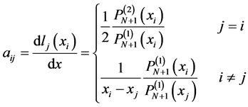
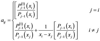
Similarly, the following expression defines aJI [29] [30]
 (44)
(44)
where
 (45)
(45)
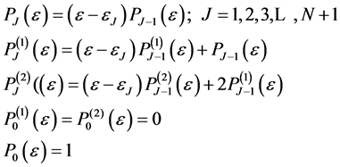
Recall that the elements of the matrix can be generated from the following Lagrange polynomial
 (46)
(46)
For i = j, the elements here refer to the leading diagonal of the matrix to be generated.
For i ≠ j, the elements here refer to all other elements of the matrix.
Also, the following recurrence relations are defined below
 (47)
(47)
For 
The following substitutions and manipulations will now be made to redefine Equation (46).
Substituting the recurrence relations into Equation (46) yields
 (48)
(48)
Now, some terms will be cancelled out.
Since j = i, (xi − xj) = 0,
And
(xj − xj) = 0
 (49)
(49)
The above becomes
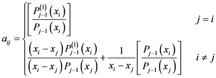 (50)
(50)
This becomes
 (51)
(51)
Rewriting the above in terms of epsilon, (ε)
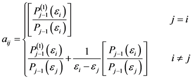 (52)
(52)
The matrix now looks like this


 (53)
(53)
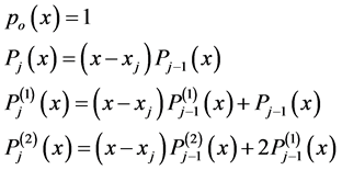
The recurrence relations below will again be used to evaluate the terms of the matrix
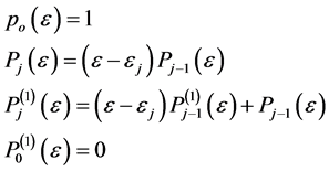 (54)
(54)
Let e assume the range e = [0:0.01:0.09]
where
 (55)
(55)
 (56)
(56)
 (57)
(57)
3. Results
The reservoir response, as predicted by the simulation on the basis of the theory of coherence, is compared with the numerical predictions obtained using traditional finite difference method and orthogonal collocation. For the case studies, data from a hypothetical well and an existing Nigerian well data were used for the validation of the simulation design. The main objective of these case studies has been to demonstrate that the mathematical techniques of orthogonal collocation, finite difference and coherent theory in the context of simulator design can be used to obtain wave behaviour in a reservoir. A gradually increasing level of complexity is introduced, repre- senting a range of systems from aqueous phase flow, to surfactant chromatography in two phase flow and to surfactant chromatography in two dimensional porous medium. The initial and injected surfactant compositions corresponding to Cases 1, 2 and 3 are shown in Table 5. The rock and fluid properties are listed in Tables 1-4. These properties are assumed uniform for convenience.
The two fluid phases consisted of a water phase and an oil phase, which, for convenience are considered incompressible. The density of oil, the viscosity of oil, the salinity of water, and the formation volume factor of oil and water are listed in Table 2. All cases mentioned above were run by using anionic sodium dodecyl sulfate (SDS) and cationic dodecyl pyridinium chloride (DPC) as surfactants.
The system of equations is complete with the equations representing physical properties of the fluids and the rock. Physical properties described here are: 1) phase behaviour; 2) interfacial tension between fluid phases; 3) residual phase saturations; 4) relative permeabilities; 5) rock wettabiliy; 6) phase viscosities; 7) capillary pressure; 8) adsorption and 9) dispersion. From a physico-chemical point of view, there are three components—wa- ter, petroleum and chemical. They are in fact, pseudo-components, since each one consists of several pure components. Petroleum is a complex mixture of many hydrocarbons. Water is actually brine and contains dissolved salts. Finally, the chemical contains different kinds of surfactants.
These three pseudo-components are distributed between two phases—the oleic phase and the aqueous phase. The chemical has an amphiphilic character. It makes the oleic phase at least partially miscible with water or the aqueous phase partially miscible with petroleum.
Interfacial tension depends on the phase behaviour as the surfactant partitions between the two phases. Residual phase saturation decreases as interfacial tension decreases. Relative permeability parameters depend on residual phase saturations. Phase viscosities are functions of the volume fraction of the components in each fluid phase. Therefore, the success or failure of surfactant flooding processes depends on phase behaviour. Also, phase behaviour influences all the other physical properties, and each of them, in turn influences oil recovery.
For a two-phase flow of water and oil, where no surfactant partitions into the oleic phase, the same scenario is obtained as the one dimensional injection for Cases 1 and 2. The bed has an initial water saturation of 0.3, and is flooded with an aqueous surfactant solution. The numerical profiles agree with the coherent wave profiles. The effect of the two-phase flow is to elongate the waves, leading to a larger region of constant state and earlier breakthrough of the fast wave.
Table 5. Conditions for case studies of surfactant chromatography Hankins and Harwell [25] .
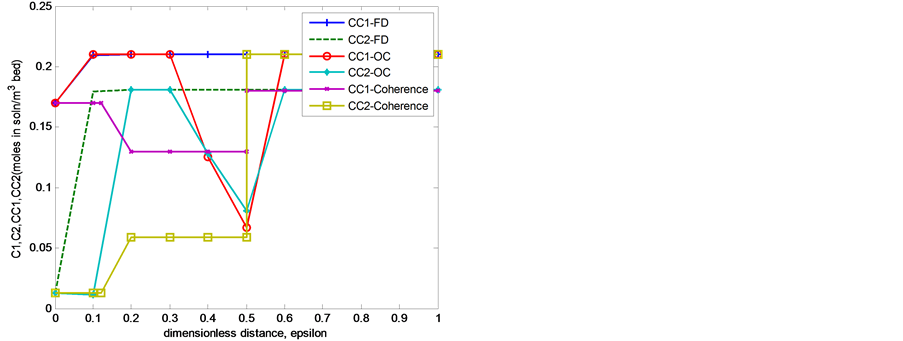
Figure 1(a) is the result obtained for solving Equation (4) using the three methods finite difference, orthogonal collocation, coherent theory. The graph is for the composition profile for one dimensional two-phase chromatography initially equilibrated with a composition C1 = 0.21, C2 = 0.181 and is then injected with a composition C1 = 0.17, C2 = 0.013 (Riemann type problem Case 1, (refer to Table 5)). In Figure 1(a), the profile C1 of finite difference shows a steady rise from C1 = 0.17 to C1 = 0.21 and then remain constant at this concentration. The profile C1 of the orthogonal collocation increases steadily from C1 = 0.17 to C1 = 0.21 at distance 0.1 epsilon maintaining a constant state to distance 0.3 epsilon. After this, it started declining from C1 = 0.21 to C1 = 0.07 at distance 0.5 epsilon before rising back to attain a constant state with the finite difference. The profile C1 of the coherent theory on the other hand started with a constant state, then declined before it reaches a constant state and then rises again to attain another constant state with the other profiles. Similarly, the profile C2 of finite difference increased steadily from C2 = 0.017 to a constant state of C2 = 0.18. The orthogonal collocation for C2 starts at C2 = 0.01 for a short constant state and then rises steadily to C2 = 0.18 to attain another short constant state from 0.2 to 0.3 epsilon. From here it depressed to C2 = 0.07 before rising back to C2 = 0.18 and then attain a constant state with finite difference. The profile C2 of coherent theory starts with a short constant state, then in- creases readily to C2 = 0.05 for another constant state from where it rises up to the final region of constant state with the other profiles.
 (a)
(a)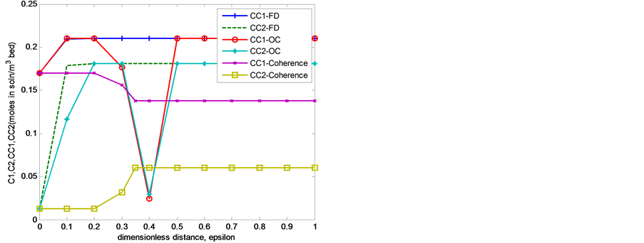
 (b) (c)
Figure 1. (a) Case 1. C1, C2 vs epsilon at τ = 0.5. Bed composition profile for one-dimensional two-phase chromatography; Case 1, at one-half pore volume injected. The plots are for three methods: Orthogonal collocation (OC), finite difference (FD) and coherent theory (CT); (b) Case 1 C1, C2 vs epsilon at τ = 1.0. Bed composition profile for one-dimensional two-phase chromatography; Case 1, at one pore volume injected. The plots are for three methods: Orthogonal collocation (OC), finite difference (FD) and coherent theory (CT). (c) Case 1 C1, C2 vs epsilon at τ = 2.0. Bed composition profile for one-dimensional two-phase chromatography; Case 1, at two pore volumes injected. The plots are for three methods: Orthogonal collocation (OC), finite difference (FD) and coherent theory (CT).
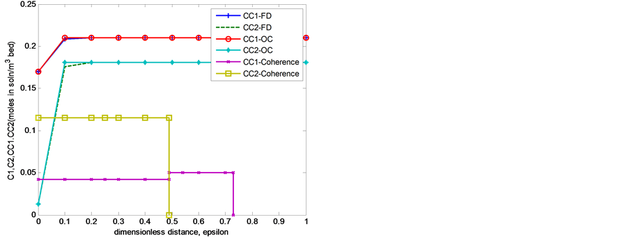
Figure 1(b) shows the result obtained for solving Equation (4) by using orthogonal collocation and finite difference as the numerical technique. The graph is for the bed composition profile for one dimensional two-phase chromatography for Case 1 at one pore volume injected. In this case also, the adsorbing porous medium is initially equibrated with a composition C1 = 0.21, C2 = 0.181 (concentrations normalized as moles in solution per m3 of bed) and is then injected with a composition C1 = 0.17, C2 = 0.013 (Riemann-type problem: Case 1 (refer to Table 5). The profile C1 for finite difference indicates a rise in concentration from C1 = 0.17 to 0.21 after which the concentration maintained a constant state. The profile of C1 for the orthogonal collocation also rise from C1 = 0.17 to C1 = 0.21 but falls to 0.03 epsilon at distance 0.4 epsilon and then increased thereafter to constant state as maintained in the C1 profile for finite difference. The profile C1 of coherent theory started with a constant concentration and then decreased gradually to attain another region of constant state. The profile C2 of finite difference increased steadily from C2 = 0.02 to attain constant state at 0.18 epsilon. Also the profile of C2 of the orthogonal collocation increases gradually from C2 = 0.02 to C1 = 0.18 at distance 0.2 for a short constant state and then decline to a low value of C2 = 0.02 at distance 0.4 epsilon before rising back to reach a constant state with the finite difference profile. The profile C2 of coherent theory started with a constant state and gradually rises to a constant state
The bed composition profile for one dimensional two-phase chromatography for Case 1 at two pore volume injected is shown in Figure 1(c). This is the result obtained for solving Equation (4) by using these three techniques; finite difference, orthogonal collocation and coherent theory. The adsorbing porous medium is initially equibrated with a composition C1 = 0.21, C2 = 0.181 (concentrations normalized as moles in solution per m3 of bed) and is then injected with a composition C1 = 0.17, C2 = 0.013 (Riemann-type problem: Case 1 (refer to Table 5)). The profile C1 of finite difference and the profile C1 of orthogonal collocation indicate that there is steady increase from C1 = 0.17 to C1 = 0.21 at distance 0.1 epsilon and then attained a constant state for both profiles. However, the profile C1 of coherent theory shows a constant state of concentration at C1 = 0.04 before having a self sharpening shock at C1 = 0.05, and eigenvalue λ = 0.499. It then continues at this constant state and then decreased to zero at distance 0.73. Similarly, the profile C2 of finite difference shows a steady rise from C2 = 0.02 to C2 = 0.18 and then maintained a constant state. Also, the profile C2 for orthogonal collocation, follows the same pattern, which indicates an increase from C2 = 0.02 to C2 = 0.18 and then attained a constant state. The orthogonal collocation profiles match the finite difference profiles. However, the profile C2 of coherent theory shows a constant state of concentration but has no self sharpening at C2 = 0.00 in this case before its termination at distance 0.499 epsilon.
Figure 2(a) shows the bed concentration profiles for one dimensional two-phase chromatography for Case 2 at one pore volume injected in the porous medium initially devoid of surfactant and then injected with a mixture C1
 (a) (b)
Figure 2. (a) Case 2, C1, C2 vs epsilon at τ = 1.0. Bed composition profile for one-dimensional two-phase chromatography; Case 2, at one pore volume injected. The plots are for three methods: Orthogonal collocation (OC), finite difference (FD) and coherent theory (CT); (b) Case 2. C1, C2 vs epsilon at τ = 2.0. Bed composition profile for one-dimensional two-phase chromatography; Case 2, at two pore volumes injected. The plots are for three methods: Orthogonal collocation (OC), finite difference (FD) and coherent theory (CT).
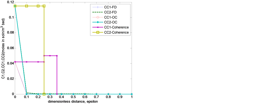
= 0.042, C2 = 0.115 (Riemann-type problem, Case 2 (refer to Table 5), with the numerical result obtained for solving Equation (4) by using three different techniques; orthogonal collocation, finite difference and coherent theory. The profile C1 of finite difference shows steady decline from C1 = 0.04 to a constant state, the same as for orthogonal collocation. However, the profile C1 of coherent theory shows a constant state of concentration at C1 = 0.04 before having a self sharpening shock at C1 = 0.048 and eigenvalue λ = 0.26. It then continues with a constant state and decreased to zero at distance 0.37. The profile C2 of finite difference decreased steadily from C2 = 0.119 to C2 = 0.001 and then to a constant state as for C1; a. similar behaviour was observed for orthogonal collocation. Again, the profile C2 was different for coherent theory where a constant state was initially observed with no self sharpening at C2 = 0.00.
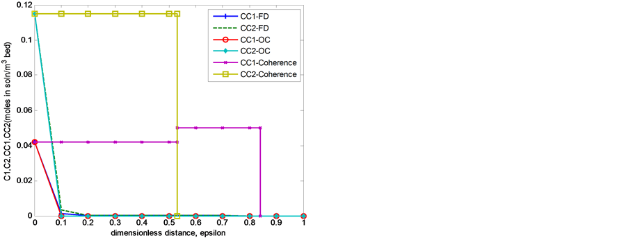
The bed composition profile for one dimensional two-phase chromatography for Case 2 at two pore volume injected is shown in Figure 2(b). This is the result obtained for solving Equation (4) by using the three techniques; finite difference, orthogonal collocation and coherent theory. The profile of C1 for finite difference shows steady decline from C1 = 0.04 to a constant state; similar behaviour was observed for orthogonal collocation. A difference was again observed for the profile C1 of coherent theory where the profile shows a constant state of concentration at C1 = 0.04 before having a self sharpening shock of C1 = 0.046, and eigenvalue λ = 0.53. It then continues with a constant state and decreased to zero at distance 0.84 epsilon. The profile C2 of finite difference decreased steadily from C2 = 0.119 to C2 = 0.001 and then to a constant state as for C1; a similar behaviour was observed for orthogonal collocation.
In Figure 2(b), the profiles C1 of orthogonal collocation, finite difference and coherent theory follow the same pattern as that in Figure 2(a). Similarly, the profiles C2 of finite difference, orthogonal collocation, coherent theory in Figure 2(a) have the same pattern as those in Figure 2(b).
There are two regions of moderate change corresponding to two “fronts”. These are the leading edge of the surfactant and the solubilization (or miscible) front as the concentrations jump to their injected values. Physically, this region corresponds to the very rapid increase in the relative permeability of the aqueous phase due to the decrease in interfacial tension. This is, of course, what the surfactant is designed to do, and is a physically desirable feature of the process.
Oil Recovery
It is necessary to generate averaged relative permeability curves which are functions of the thickness averaged water saturation and use these in the oil recovery calculations. At a constant temperature, the oil and water viscosities have fixed values and are strictly functions of the water saturation as related through the relative permeabilities.
Table 6 shows the values of water saturation and viscosities for Case A (hypothetical reservoir data) and Case B (Nigerian reservoir data) from which the relative permeability curves for cases A and B are plotted respectively (see Figure 3 and Figure 4).
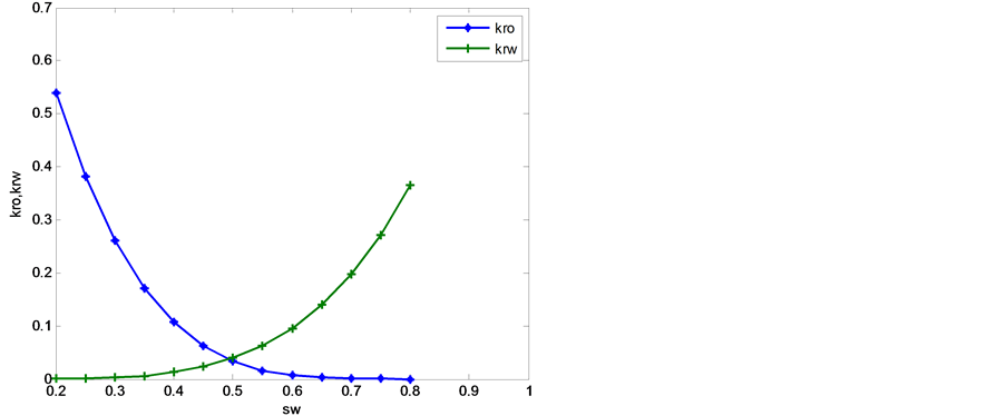
Figure 3. Graph of kro and krw against Sw for Case A. Effective and corresponding relative permeability as functions of water saturation for Case A.
![]()
Figure 4. Graph of kro and krw against Sw for Case B. Effective and corresponding relative permeability as functions of water saturation for Case B.
Table 6. Water saturations and viscosities for Cases A and B.
Table 7 shows the values of fractional flow and water saturation in the reservoir for Case A and Case B. These values are used to obtain fractional flow plots for both Cases A and B as shown in Figure 5.
Figure 3 shows the saturation dependence of the effective permeabilities of oil and water. The plot shows both permeabilities as functions of the water saturation alone since the oil saturation is related to the water saturation by a simple relationship So = 1 − Sw. On the effective permeability of water (krw) curve, Sw = Swc = 0.2 on the Sw axis. At Sw = 1, kw= 1.0. Similarly, for the effective permeability for oil curve Sw = Swc = 0.2 At Sw = 1, kro = 0.55. The curves are used to describe the displacement of oil by water taking into consideration the manner in which the fluid saturations are distributed with respect to thickness as they simultaneously move through the reservoir. Surfactants dissolved in minute quantities of water have significant effect on displacement of oil and in-
![]()
Figure 5. Fractional flow plots for oil-water viscosity ratios. Graph of fw against sw.
Table 7. Fractional flow and water saturation for cases A and B.
crease the oil saturation above Sor. This result in moving from point Sor, Kor = 1 on the normal relative permeability curve thereby raising the saturation above the residual level to render the oil mobile.
Figure 4 shows the saturation dependence of the effective permeabilities of oil and water. The plot shows both permeabilities as functions of the water saturation alone since the oil saturation is related to the water saturation by a simple relationship So = 1 − Sw. On the effective permeability of water (krw) curve Sw =Swc = 0.2 on the Sw axis. At Sw = 1 kw= 0.7. Similarly, for the effective permeability for oil curve Sw = Swc = 0.2 at Sw = 1 kro = 1.0 Also, the curves are used to describe the displacement of oil by water taking into consideration the manner in which the fluid saturations are distributed with respect to thickness as they simultaneously move through the reservoir. Surfactants dissolved in minute quantities of water have significant effect on displacement of oil and increase the oil saturation above Sor. This result in moving from point Sor, Kor = 1 on the normal relative permeability curve thereby raising the saturation above the residual level to render the oil mobile.
If we compare Figure 3 and Figure 4 for the hypothetical data and the Nigerian oil data, we notice the residual oil saturation curve of Figure 4 being shifted to the right of the residual oil saturation curve of Figure 3. So, when the surfactant contacts the residual oil, the surfactant dissolves in it and then raises the saturation above the residual level. Also, there is a significant reduction in the surface tension between these enlarged oil droplets and the displacing water. Moreover, since the relative permeability of the oil increases from zero upwards, then the residual oil becomes more mobile for the Nigerian oil (Figure 4) than that in Figure 3 (the hypothetical oil). This results in more oil being recovered from Figure 4 than in Figure 3.
Fractional flow values for A and B obtained with the application of Welge’s technique at breakthrough are listed in Table 7. Also, the fractional flow curve drawn using the averaged relative permeability curves and the Buckley Leverett/Welge technique to calculate oil recovery is shown in Figure 5. This figure shows the fractional flow plots for different oil water viscosity ratio for cases A and B. The fractional flow plot exhibit the characteristic S shape with saturation limits, Swc and 1 ‒ Sor, between which the fractional flow increases from zero to unity. The tangent to the fractional flow curve from the point Sw = Sw; fw = 0 has a point of tangency with co-ordinates Sw = Swbt = 0.50; fw = fw|swf = fwbt = 0.86 for Case A and Sw = Swbt = 0.61; fw = fw|swf = fwbt = 0.91 for Case B (refer to Table 8). The extrapolated tangent intercept the line fw = 1 at the point fw = 1; Sw = Swbt = 0.55 for Case A and at point fw = 1; Sw = Swbt = 0.65 for Case B. (refer to Table 8). Table 9 shows values of shock front, end point relative permeabilities and mobilities ratio obtained from Figure 5 by applying Welge’s technique.
Figure 6 shows the oil recovery in a resevoir as a function of dimensionless water injected for both casE A (hypothetical resevoir) and Case B (Nigerian reservoir). The graph is plotted from the caiculated values of fwe, Wid and Npd shown in Table 10 and Table 11 The graph shows that the oil recovery curve for Case B rises above that of Case A even with less injected pore volume. This show that the break through occurred much earlier for B. The oil recovery for Case A reservoir is 0.61 while that for Case B reservoir is 0.73.
![]()
Figure 6. Dimensionless oil recovery as a function of dimensionless injected pore volume. Comparison of the oil recoveries obtained for Case A and Case B reservoirs.
Table 8. Flood front saturation values.
Table 9. Values of shock and end point relative permeabilities.
Table 10. Cumulative oil recovery as function of wid for Case A.
Table 11. Cumulative oil recovery as function of wid for Case B.
The tangent to the fractional flow curve from the point Sw= Swc, fw= 0 gives the coordinates to obtain parameters to calculate the oil recovery for both Cases A (Hypothetical data) and B (Nigerian oil data).
The values in Table 5 and Table 6 were used to generate the plots of dimensionless oil recovery as a function of injected pore volume in Figure 6. This shows the oil recoveries for both Case A and B reservoirs.
In Figure 6, plot of the oil recovery of reservoir A is compared with that of plot of oil recovery for reservoir B. The comparison shows that, the breakthrough occurs much earlier for Case B, the ultimate recovery is obtained for a much smaller throughput of injected pore volume and sooner than for Case A. The oil recovery for Case A reservoir is 0.61 while that for Case B reservoir is 0.73
4. Discussion of Results
The ultimate objectives of the simulator designed in this work are two-fold:
1) The prediction of the appropriate surfactant concentrtion necessary for the required enhanced oil recovery from reservoirs, and
2) The volume of recovered oil from the reservoir using the hypothetical reservoir oil data and Nigerian oil reservior data.
With regard to item 1 above, the basic physical principle employed by the simulator is that of mass conservation. Usually those quantities are conserved at stock tank conditions and related to reservoir fluid quantities through the pressure dependent parameters. The profiles of three cases (1, 2, 3) in one dimensional aqueous phase chromatography and two-phase chromatography for one, one-half, and two pore volume injected were developed using simulated solutions to model equations. These equations were solved by finite difference (FD), orthogonal collocation (OC) and coherent theory (CT).The use of these methods permit the determination of the relative efficiency of the methods and how well they predict the complex characteristics of the enhanced oil recovery process. We will now discuss the significant results of this work regard to items 1 and 2 above.
We did find out that:
1) Injecting a mixture of low concentration aqueous surfactant composition into adsorbing porous medium that is initially injected with high concentration aqueous surfactant composition. This variation may exist in the initial profile or be generated by injection. The initial fluid or previously injected fluid has the composition downstream of the change in amount while the newly injected fluid has the composition upstream of the original variation. The composition route along the bed follows the slow path from the injected composition and then switches to the fast path which leads to the previously injected compòsition. The route passes along paths and follows the paths in the sequence of increasing wave velocities.
2) Injecting a mixture of an aqueous composition into a porous medium, initially devoid of surfactant, the expected composition is a self sharpening shock wave. The steepness in all the profiles generated by finite difference (FD), orthogonal collocation (OC), and coherent theory (CT) confirms the self sharpening behaviour. It may be noted in all cases of these nature the waves trajectories gradually fall, as a result of a gradual increase in the associated eigenvalues of the waves as salinity increases. The finite difference (FD) and orthogonal collocation (OC) response essentially agrees with the coherent method except for a slight curvature. This is because the finite difference (FD) and orthogonal collocation (OC) are no longer a good approximation to the shock The consequence of this steepening is that the flows are sharpening, so that they break through both earlier and over a smaller injected volume. For the dependent variables such as component concentration, common velocity exists at each point in the wave, and the associated composition route remains unchanged and the same during relative shifts of waves associated with other dependent variable waves as shown in all the methods. This is in agreement with Helferich [4] .
Injecting a mixture of high concentration of surfactant into adsorbing porous medium that is initially injected with low concentration aqueous surfactant composition yield two types of path. The slow and fast paths. The slow path eigenvalues are close to the fast path with eigenvalues of 1 and the effect of dispersion results in the merging of the two waves. This is due to their spatial positions, and loss of intermediate region of constant state. This region later reappear with less dispersion.
3) For a system of two-phase (aqueous and oleic) flow of water and oil in which there is no surfactant partitions into the oleic phase. The effect of two phase flow elongated the wave, leading to a larger region of constant state and earlier breakthrough of fast wave. The shock and wave composition route are identical to that of aqueous phase and has a unique composition path grid which is independent of the saturation of the flowing phases. This is similar to system of a two-phase (aqueous and oleic) flow in which two water soluble components partition between the aqueous and a solid adsorbent phase [20] .
4) When surfactant partitions into the oleic phase, the effect is that the adsorption of the surfactant in the solid phase results in the formation of micelles which then break away from the solid phase and move much faster than the surfactant in the oleic phase. The domination of the micelle formation in the aqueous phase is the general effect for both slow and fast phases. The presence of the two partitioning components does not alter the fractional flow relations fj(Sj) for the two phases. The sum of the aqueous and oleic phase saturations must add up to one wave of the saturation variables
5) The solutions observed with the coherent theory (CT), finite difference (FD) and orthogonal collocation (OC) were not too dissimilar; they were however, not exact. The slight differences are due to assumed discrete values used for each method. The coherent wave fronts match the other two methods at their points of turning, where the effective wave dispersion is zero.
The simulation results of the predicted profiles by the coherent theory (CT), finite difference (FD) and orthogonal collocation (OC) techniques illustrate the typical effects of a pattern flood such as the early breakthrough of the oil bank and the long tail on the oil surfactant curves. The results show only significant deviations in some sections. The only significant difference beween the coherent theory (CT) and finite difference (FD) results is that the finite difference (FD) profiles are continous while the coherent profiles exhibit discontinous. More oscillations are evident in the orthogonal collocation (OC) solution profiles. This indicates that orthogonal collocation (OC) solution is sensitive to oscillation than other methods. This is particularly noticeable in the curves following breakthrough. The finite difference (FD) is considerably more dissipative and therefore the small oscillations are absent. Also, the coherent suppresses oscillation and is less dissipative. These findings are beyond the findings of Hankins and Harwell [20] . For, the work of Hankins and Harwell [20] did not show any of these new findings discussed here.
6) Several simulations were made to evaluate the dependence of oil recovery on slug size for a given amount of injected surfactant. This is an important design factor and has been studied by many people for some years. It is generally thought that a large dilute slug will be better in a heterogeneous reservoir. This seems intuitively correct since a small slug would seem to be proportioned into the lowest permeabilities in such a small amount that little if any oil recovery from those parts of the reservoir could be expected. This is by itself would not be an unreasonable strategy provided portion of the reservoir which is the target only, The dependence of oil recovery on slug size for a given amount of injected surfactant or for a fixed product of slug size time’s surfactant concentration indicates that the more surfactant injected the more oil recovered. So the effect of surfactant slug size is predictable. The effect of surfactant concentration is also predictable in the same manner as more oil is recovered for increase in surfactant concentration injected.
7) The oil recoveries are attributed to the reduction of oil-water interfacial tension. Residual oleic phase saturation for the water-oil surfactant system depends on interfacial tension Oil initially at residual saturation is displaced by injection of surfactant solution. Through a complicated and highly non-linear function of the phase concentrations, the surfactant solution lowers the oil-water interfacial tension, and thus mobilizes the trapped oil. Three separate phases can form when such fluids displace oil-water mixtures. There are two regions of moderate change corresponding to two “fronts”. These are the leading edge of the surfactant and the solubilization (or miscible) front as the concentrations jump to their injected values. Physically, this region corresponds to the very rapid increase in the relative permeability of the aqueous phase due to the decrease in interfacial tension. This is, of course, what the surfactant is designed to do, and is a physically desirable feature of the process. Oil trapped after water flooding is displaced by the injection of a slug of surfactant solution. The surfactant solution lowers the oil-water interfacial tension and, thus mobilizes the trapped oil. Therefore, residual oleic phase saturation for the water-oil-surfactant system depends on interfacial tension.
The complexities could not have been detected by using only the coherent technique as used by Hankins and Harwell [25] . This is a major accomplishment of this work. Not only was the discontinuities discovered by this work, it also provides an insight into the complex behaviour of enhanced oil recovery process.
We will now focus on the ultimate objective of this work, which is the volume of oil recovery achievable by our simulator.
Almost no change occurred was observed in the oil recovered as the slug size changed from one percentage of the pore volume to another, provided the salinity gradient was exactly the same for all runs. The implication is that slug size per se makes almost no difference over the range of typical slug sizes used in practice. Other factors such as the mobility control do matter and may be affected by the type of slug used and, from the point of view of chemical of injected surfactant.
The dependence of oil recovery on slug size for a given amount of injected surfactant indicates that the more surfactant injected the more oil is recovered. This is because an injected surfactant disperses into oil and water, then lowers the interfacial tension thereby mobilizing more immobile oil. This is continued until the surfactant is diluted or lost due to adsorption by the rock. For significant incremental oil recoveries, several orders of magnitude reduction is needed. Hence, large quantities of surfactant are required for reduction of the interfacial tension to produce the desired effect. So, the effect of surfactant slug size is forecastable. The effect of surfactant concentration is also predictable in the same way as more oil is recovered for increases in surfactant concentration injected.
The oil recovered in the reservoir Case A (hypothetical data) is lower than that of reservoir Case B (Nigerian oil data). The comparison shows that the breakthrough occurs much earlier for Case B, the ultimate recovery is obtained for a much smaller throughput of injected pore volume and sooner than for Case A.
5. Conclusions
The applicability of the simulator for the solution of the model equations of multiphase, multicomponent flow and transport in a reservoir has been demonstrated using orthogonal collocation solution. The results of the orthogonal collocation solution were compared with those of finite difference and coherence solutions. The results obtained using this methodology revealed certain features unobserved by previous investigators [25] . The results indicate that the concentration of surfactants (C1, C2) for orthogonal collocation appears to show more features than the predictions of the coherence solutions and finite difference. The reason for the difference is the subject of continuing study. It is unlikely that the coherence approach alone could ultimately accommodate the comple- xities required for a full field reservoir simulator.
It is obvious that the coherent routes for the compositions of adsorbing surfactants correspond to the simpler case of aqueous phase chromatography, with modified eigenvalue. This observation also holds for “shock” waves. The existence of a partially coherent solution makes the prediction of reservoir response much more straightforward. However, the “partially” coherent solution only exists if surfactants do not partition into the oleic phase and fractional flow is not a function of surfactant composition; should either occur, a globally coherent solution may still be found, but the solution is more complex and difficult to handle. There is no equivalence of partial coherence in the orthogonal and finite difference methods. In these lie the possibility of the differences in the concentration profiles predicted by the three numerical techniques. Again, the use of the orthogonal collocation and finite difference solution provides easier solution to future possible problems that may arise as the simulator is being used.
The dependence of oil recovery on slug size for a given amount of injected surfactant indicates that the more surfactant that is injected, the more oil is recovered. For significant incremental oil recoveries, several orders of magnitude interfacial tension reduction are needed. Hence, large quantities of surfactant are required to produce the desired effect of high oil recovery.
The predicted oil recovery for the Nigerian oil reservoir is higher than that predicted for the hypothetical reservoir data. The displacement is stable in the Nigerian oil reservoir due to the moderate value of the oil/water viscosity instead of the other reservoir with high value of oil/water ratio.
References
- Glimm, J., Lindquist, B., McBryan,
- Ewing,
- Zheng, C. (1993) Extension of the Method of Characteristics for Simulation of Solute Transport in 3 Dimensions. Groundwater, 31, 456-465. http://dx.doi.org/10.1111/j.1745-6584.1993.tb01848.x
- Helfferich, F.G. (1981) Theory of Multicomponent, Multiphase Displacement in Porous Media. Society of Petroleum Engineers Journal, 21, 51-62. http://dx.doi.org/10.2118/8372-PA
- Lake,
- Dezabala,
- Hirasaki, G.J. (1981) Application of the Theory of Multicomponent, Multiphase Displacement to Three-Component, Two-Phase Surfactant Flooding. Society of Petroleum Engineers Journal, 21, 191-204. http://dx.doi.org/10.2118/8373-PA
- Pope,
- Lake,
- Helfferich,
- Araque-Martinez, A. and Lake,
- Harwel,
- Helset,
- Cirpka,
-
- Fayers,
- Claridge,
- Larson, R.G. (1979) The Influence of Phase Behaviour on Surfactant Flooding. Society of Petroleum Engineers Journal, 411-422. http://dx.doi.org/10.2118/6774-PA
- Lake,
- Hankins,
- Siggel, L., Santa, M., Hansch, M., Nowak, M., Ranft, M., Weiss, H., Hajnal, D., Schreiner, E., Oetter, G. and Tinsley, J. (2012) A New Class of Viscoelastic Surfactants for Enhanced Oil Recovery. SPE Improved Oil Recovery Symposium, 14-18 April 2012, Tulsa, Paper ID: SPE-153969-MS. http://dx.doi.org/10.2118/153969-MS
- Xu,
- Leach,
- Harwell,
- Hankins,
- Oyedeko,
- Trogus,
- Helfferich, F.G. (1986) Multicomponent Wave Propagation: Attainment of Coherence from Arbitrary Starting Conditions. Chemical Engineering Communications, 44, 275-285. http://dx.doi.org/10.1080/00986448608911360
- Villadsen,
- Villadsen,
NOTES

*Corresponding author.