ABSTRACT

The determination of water saturation is a key step for the reservoir characterization and prediction of future reservoir performance in terms of production. The importance of water saturation has been further identified when the reservoirs refer to rocks with low porosity and permeability such as shale and tight formations. In this communication, two advanced artificial intelligence strategies consisting of least square support vector machine (LSSVM) and gene expression programming (GEP) have been applied in order to develop reliable predictive models for the calculation of water saturation of shale and tight reservoirs. To this end, an extensive core and log data bank has been analysed from 12 wells of a Mesaverde group tight reservoir located in the largest Western US. The results indicate that the estimated water saturation data by the models developed in this study are in satisfactory agreement with the actual log data. Furthermore, new methods proposed in this study are useful for the characterization of shale and tight reservoirs and can be applied to the relevant software.

Keywords:

Shale, Petrophysical Properties, Water Saturation, GEP, LSSVM

1. Introduction

The reservoir characterization is a fundamental task for the determination of future reservoir performance. A large number of errors may enter the calculations associated with a future prediction of reservoir performance if there is no accurate and appropriate reservoir characterization which can cause the lose of the important values of reserves estimations and hydrocarbon production, etc. [1]. In particular, the water saturation has significant effects on shale reservoir performance [2] [3]. Accurate estimation of water saturation is accounted as one of the most challenging computations associated with petrophysical properties. In reservoir characterization, the determination of water saturation is a key step for the prediction of future reservoir performance in terms of production. Furthermore, the value of water saturation is needed in calculations related to the original oil and gas place so that the difference in water saturation calculated may lead to considerable differences in these volumes. The importance of water saturation has become more apparent when the reservoirs refer to rocks with low porosity and permeability such as shale and tight formations. As a result, the shales make up a large proportion of the rocks with many challenges and complexities. The availability of detrital clay minerals in pores, reservoir heterogeneities in the directions vertically and laterally, considerable formation thickness, over-pressures condition, the existence of free water zone independently, and the intercalation and co-existence of source rocks with reservoir rocks could be accounted as main differences between the shale tight and conventional reservoirs [4].

Over the years, many attempts have been carried out for accurate calculation of formation water saturations. Furthermore, there are few studies to estimate water saturation of shale and tight reservoirs. Fertl and Hammack [5] conducted a comparative study of the different methods to calculate water saturation of shaly sandstone reservoirs utilizing the actual field data. The comparative analysis conducted by them indicated the practical applications of these different techniques to the interpretation of shaly pay sands.

Al-Blushi et al. [6] proposed some predictive models to calculate water saturation based on log data. They used artificial neural network (ANN) methodology to develop their model for two Middle Eastern sandstone reservoirs. The results indicated that the model developed based on ANN strategy is capable to predict water saturation of Middle Eastern reservoirs studied. Kenari and Mashohor [7] used machine learning approach to propose an intelligent model for the prediction of water saturations. To this end, they used well log data from un-cored well. The results revealed that the intelligent method employed is accurate and rapid for the prediction of water saturation. Amiri et al. [8] developed an ANN model to estimate water saturation in tight and shale gas reservoir. They also used the imperialist competitive algorithm as optimization methodology to couple with the ANN algorithm. The results demonstrated that the model developed based on the neural network and imperialist competitive algorithms outperform the conventional method compared in their study.

As a result, the previously published models available in the literature fail to cover a wide range of petrophysical properties to estimate water saturation. Furthermore, the literature models have not been proposed on the basis of large numbers of water saturation data points. As a result, the prediction of water saturation by the literature models requires time-consuming calculations, reading graphs, optimization of the coefficients, etc. Therefore, the development of simple-to-use predictive models as well as empirically derived methods is needed. In this study, a large and extensive data bank is used, including more than four thousands petrophysical data points for the development of a reliable artificially intelligent based model which is based on the least square support vector machine (LSSVM) and an empirically derived method using gene expression programming (GEP) algorithm. Additionally, the most important error parameters are calculated to visualize the accuracy of the models proposed in this study as well as graphical error analysis including scatter diagram and contour map.

2. Database

A literature survey on the previously published researches demonstrated that true formation resistivity (R_t), porosity induced by neutron log (PHID), porosity induced by density log (PHIN), effective prosity from density log (PHIDE), effective prosity from neutron log (PHINE), effective porosity induced by density and neutron logs (PHIDNE), effective porosity (PHIE), total porosity (PHIX), bulk density (RHOB), photoelectic (PE), and volume of shale from gamma ray (V_sh) are known as the most effective parameters for the calculation of water saturation (S_w) [6] [7] [8] [9] [10]. Therefore, a large and comprehensive data bank including the petrophysical properties noted above is provided in this study in order to develop reliable models for accurate estimation of water saturation of shale and tight gas reservoirs. To this end, the core and well log data [8] from 12 wells of Mesaverde group tight reservoir located in the largest Western US has been applied for the model development. More than 4000 data points has been considered from one of the tight gas sand basins in this study. These data show that Sw does not have a strongly linear relationship with individual parameter: PHIE, V_sh, R_t, PHIN, PHIDE, PHIDNE. Therefore, all of the paramters are correlated with collectively. The petrophysical properties which have the highest effects on the water saturation data available in the data bank are considered as input parameters for the model development. Table 1 summarizes the ranges of the most effective petrophysical properties as well as water saturation data available in the data bank provided.

3. Development of Models

3.1. Least Squares Support Vector Machine Model

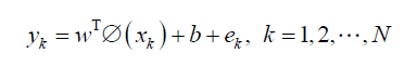
Least squares support vector machines are least squares forms of support vector machines (SVM), which are a set of associated supervised learning methods that investigate data and identify patterns, and that are used for sorting and regression analysis offered by Suykens et al. [11] [12] [13]. In LS-SVM a linear approximation is prepared in kernel induced feature space. By considering a data set $\left(x_i,y_i\right),i=1,2,\cdots ,N$ , with input data $x_i\in R$ and output data $y_i\in R$ , the regression model can be established as follows [13] [14] [15] :

(1)

In these equations w characterizes the linear regression (regression weight), T is symbolic of the transpose matrix, e is training items regression error, b is the model linear regression intercept, and shows the feature map. The cost function of LSSVM algorithm, Q_LSSVM is calculated below [12] [13] [14].

(2)

is the relative weight of the regression errors summation compared to the regression weight. By assistance of Lagrange function, the regression weight normally is showed as follows [16] [17].

(3)

In which is defined as.

(4)

With the assumption of linear regression between independent and dependent LSSVM variables, Equation (1) can be re-written as [14] [16].

(5)

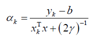
With the subsequent equation the Lagrange multipliers, can be considered as [12] [13] [17].

(6)

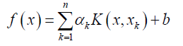
By means of Kernel function the first linear regression equation will be changed into a nonlinear form [15] [16] [17].

(7)

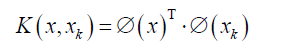
In the above equation, represents the Kernel function, made by inner product of the vectors and [13] [16].

(8)

Radial basis function (RBF) is the utmost used relation for calculating the Kernel function [14] [17].

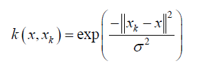(9)

Here is a decision variable. Its optimisation is controlled by an external procedure during model’s internal computations. The mean square error (MSE) definition for the LSSVM can be defined as follows [16] [17].

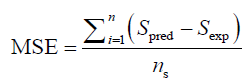(10)

where S is the water saturation, pred. and exp. stand for the predicted, and experimental or actual data, respectively, and n_s is the initial population number [16] [17].

3.2. Gene Expression Programming

Ferreira [18] developed an intelligent evolutionary algorithm called gene expression programing (GEP) which is able to construct symbolic models mathematically. In GEP approach, control parameters, function set, fitness function, terminal set, and termination condition are recognized as the key components [19]. Those parse trees are known as expression trees (ETs) for the GEP algorithm [20]. Hence, the nature of gene expression programming authorities the evolution of more complex programs composed of various substructures or subprograms so-called GEP genes. For illustrating the mathematical performance of the GEP methodology in developing symbolic models, a simple GEP-based equation counting a chromosome composed of two genes connected together by a multiplication fitness function is expressed as follows:

$\left(u\times v\right)+\left(\frac{f}{l}\right)$ (11)

where u, v, f and l express the input variables for estimating the target variable (water saturation), and ÷, × and + stand for the fitness functions.

3.3. Model Development

For developing predictive models to estimate the water saturation data using two modelling strategies viz. the LSSVM and GEP algorithms, the same input variables including PHIE, V_sh, GR, R_t, PHIN, PHIDE, PHIDNE have been considered. The database gathered should be randomly divided into two sub-sets. The first sub-set is called “Training” and the second is “Test” set which have been applied to develop models and check the prediction performance, respectively. Around 80 % of the entire data is assigned to the training set, and the rest is allocated to the test set. In this study, two important statistics error parameters have been used through a comprehensive error analysis in order to visualize the accuracy and performance capability of the developed models for the water saturation prediction. The statistical error parameters implemented in this study are squared correlation coefficient and average absolute relative deviation (AARD) as follows:

(12)

(13)

In the first stage, the LSSVM algorithm was coupled with an optimization strategy known as coupled simulated annealing (CSA) [21] [22] [23] for obtaining the optimum values of the LSSVM parameters (γ and σ²). As a result, the values tuned by the CSA technique for the LSSVM model in order to estimate the water saturation data are σ² = 1.4181 and γ = 328.2432. To propose a new empirically derived equation based on the GEP algorithm, three genes with 30 chromosomes are applied as a starting condition. Additionally, the AARD is considered as the accuracy function so that the optimal form of the newly developed model has the lowest AARD. Furthermore, a function set including power, cube root, ×, ÷, - and + is selected during applying the GEP methodology. The final model obtained by the GEP algorithm developed in this study is a simple-to-use equation with lowest possible coefficients as follows:

(14)

(15)

(16)

(17)

where S_w denotes the water saturation, PHIDNE stands for the effective porosity induced by density and neutron logs, PHIDE indicates the effective porosity from density log, PHIN shows the porosity induced from neutron zoned, PHIE is the effective porosity, V_sh expresses the volume of shale from gamma ray, and finally R_t stands for the true formation resistivity.

As a result, the optimal condition to apply the equations above is the range of the petrophysical properties used which have previously been summarized in Table 1. Furthermore, another important condition to develop the equations above is that some input parameters i.e. V_sh, PHIDE, PHIDNE, PHIE have a minimum value of zero and should not be in the denominator individually. Therefore, this condition is considered to develop the equations presented above. Although the equation proposed in this study is also applicable for calculating water saturation of conventional reservoirs, the equations proposed in this study have been developed based on the data from shale and tight reservoirs.

4. Results and Discussion

The error parameters calculated for the LSSVM model and the new method (Equation (14)) are AARD= 3% and R-squared= 0.96, and AARD= 10.6 and R-squared = 0.77. Table 2 also summarizes some calculated water saturation data by the predictive models developed in this study based on the LSSVM and GEP algorithms as well as the absolute relative deviation (ARD) for each data point studied. The results obtained indicate that the water saturation values characterized by the GEP and LSSVM models are in satisfactory agreement with the actual data. For further comparison of the performance of the models developed in this study graphically, scatter diagrams (crossplot) of the data predicted versus actual data of water saturation are sketched. Figure 1 and Figure 2 illustrate the output values obtained from the LSSVM model and the newly proposed equation against the actual data of water saturation, respectively. As is shown clearly in the Figure 1 and Figure 2, the data corresponding to the developed models are almost around the unit slope line (Y = X), revealing there is acceptable agreement between the models predictions and the actual data of data of water saturation.

Figure 3 and Figure 4 reveal the absolute relative deviation contours of the water saturation predicted by the LSSVM model and the newly proposed equation, respectively. It is evident from the figures that the models developed in this study are able to predict water saturations of shale and tight reservoir in the dataset range particularly two important parameters of true resistivity and effective porosity induced by density and neutron logs. However, the model developed in the current study could not predict the water saturation with high accuracy in the PHIDNE range of 0.1 - 0.3, and R_t range of 0 - 100. From the results obtained, it could be concluded that the methods proposed in this study (the LSSVM and GEP) can be reliable alternatives for the previously published models available in the literature as they may fail to cover a wide range of petrophysical properties to estimate water saturation, and also require time-consuming calculations, reading graphs, optimization of the coefficients, etc. As a result, the accuracy and future applicability are two main advantages of the models developed in this study. The LSSVM model could predict the water saturation data with higher accuracy than the new equation proposed. On the other hand, the equation proposed based on the GEP algorithm is more simple-to-use so that it can be used for future calculations and soft wares related to water saturation and reservoir characterization. Therefore, a combined application of both LSSVM and GEP algorithms is recommended in order to accurately predict water saturation of shale and tight reservoirs.

5. Conclusion

The current study aimed to propose reliable models for the prediction of water saturation of shale and tight gas reservoir. The modelling approaches implemented in this study were the gene expression programming, and least squares support vector machine. The results obtained in the current study indicated that the two methods developed in this study could be applied for the characterization water saturation of shale reservoirs. The R-squared error values of 0.96 and 0.77 (average absolute relative deviation (AARD) of 3% and 10.6%) were obtained for the LSSVM model and the newly proposed equation, respectively. As a result, the methods proposed by gene expression programming in this study is a capable alternative for the previously published models which require complex and time-consuming calculations.

Cite this paper

Kamari, A. and Sheng, J.J. (2018) New Methods to Calculate Water Saturation in Shale and Tight Gas Reservoirs. Open Journal of Yangtze Gas and Oil, 3, 220-230. https://doi.org/10.4236/ojogas.2018.33019

References

- 1. Alimoradi, A., Moradzadeh, A. and Bakhtiari, M. (2011) Methods of Water Saturation Estimation: Historical Perspective. Journal of Petroleum Science & Engineering, 2, 45-53.
- 2. Sheng, J.J. (2015) Enhanced Oil Recovery in Shale Reservoirs by Gas Injection. Journal of Natural Gas Science and Engineering, 22, 252-259. https://doi.org/10.1016/j.jngse.2014.12.002
- 3. Sheng, J.J., Mody, F., Griffith, P.J. and Barnes, W.N. (2016) Potential to Increase Condensate Oil Production by Huff-n-Puff Gas Injection in a Shale Condensate Reservoir. Journal of Natural Gas Science and Engineering, 28, 46-51. https://doi.org/10.1016/j.jngse.2015.11.031
- 4. Crotti, M.A. (2007) Water Saturation in Tight Gas Reservoirs. Proceedings of the Latin American & Caribbean Petroleum Engineering Conference. Society of Petroleum Engineers, Buenos Aires. https://doi.org/10.2118/107145-MS
- 5. Fertl, W.H. and Hammack, G.W. (1971) A Comparative Look at Water Saturation Computations in Shaly Pay Sands. SPWLA 12th Annual Logging Symposium, Society of Petrophysicists and Well-Log Analysts.
- 6. Al-Bulushi, N., King, P.R., Blunt, M.J. and Kraaijveld, M. (2009) Development of Artificial Neural Network Models for Predicting Water Saturation and Fluid Distribution. Journal of Petroleum Science and Engineering, 68, 197-208. https://doi.org/10.1016/j.petrol.2009.06.017
- 7. Kenari, S.A.J. and Mashohor, S. (2013) Robust Committee Machine for Water Saturation Prediction. Journal of Petroleum Science and Engineering, 104, 1-10. https://doi.org/10.1016/j.petrol.2013.03.009
- 8. Amiri, M., Ghiasi-Freez, J., Golkar, B. and Hatampourd, A. (2015) Improving Water Saturation Estimation in a Tight Shaly Sandstone Reservoir Using Artificial Neural Network Optimized by Imperialist Competitive Algorithm—A Case Study. Journal of Petroleum Science and Engineering, 127, 347-358. https://doi.org/10.1016/j.petrol.2015.01.013
- 9. Poupon, A. and Leveaux, J. (1971) Evaluation of Water Saturation in Shaly Formations. SPWLA 12th Annual Logging Symposium, Society of Petrophysicists and Well-Log Analysts.
- 10. Archie, G.E. (1942) The Electrical Resistivity Log as an Aid in Determining Some Reservoir Characteristics. Transactions of the AIME, 146, 54-62. https://doi.org/10.2118/942054-G
- 11. Yarveicy, H., Moghaddam, A.K. and Ghiasi, M.M. (2014) Practical Use of Statistical Learning Theory for Modeling Freezing Point Depression of Electrolyte Solutions: LSSVM Model. Journal of Natural Gas Science and Engineering, 20, 414-421. https://doi.org/10.1016/j.jngse.2014.06.020
- 12. Samui, P. and Kothari, D. (2011) Utilization of a Least Square Support Vector Machine (LSSVM) for Slope Stability Analysis. Scientia Iranica, 18, 53-58. https://doi.org/10.1016/j.scient.2011.03.007
- 13. Suykens, J.A. and Vandewalle, J. (1999) Least Squares Support Vector Machine Classifiers. Neural Processing Letters, 9, 293-300.
- 14. Ekici, B.B. (2014) A Least Squares Support Vector Machine Model for Prediction of the Next Day Solar Insolation for Effective Use of PV Systems. Measurement, 50, 255-262. https://doi.org/10.1016/j.measurement.2014.01.010
- 15. Ding, L.-Z. and Liao, S. (2011) Approximate Model Selection for Large Scale LSSVM. Workshop and Conference Proceedings, 20, 165-180.
- 16. Safari, H., Shokrollahi, A., Jamialahmadi, M., Ghazanfari, M.H., Bahadori, A. and Zendehboudi, S. (2014) Prediction of the Aqueous Solubility of BaSO 4 Using Pitzer Ion Interaction Model and LSSVM Algorithm. Fluid Phase Equilibria, 374, 48-62. https://doi.org/10.1016/j.fluid.2014.04.010
- 17. Mesbah, M., Soroush, E., Azari, V., Lee, M., Bahadori, A. and Habibnia, S. (2014) Vapor Liquid Equilibrium Prediction of Carbon Dioxide and Hydrocarbon Systems Using LSSVM Algorithm. The Journal of Supercritical Fluids, 97, 256-267.
- 18. Ferreira, C. (2001) Gene Expression Programming: A New Adaptive Algorithm for Solving Problems. Complex Systems, 13, 87-129.
- 19. Mostafavi, E.S., Mousavi, S.M. and Hosseinpour, F. (2014) Gene Expression Programming as a Basis for New Generation of Electricity Demand Prediction Models. Computers & Industrial Engineering, 74, 120-128.
- 20. Alavi, A.H., Gandomi, A.H., Nejad, H.C., Mollahasani, A. and Rashed, A. (2013) Design Equations for Prediction of Pressuremeter Soil Deformation Moduli Utilizing Expression Programming Systems. Neural Computing and Applications, 23, 1771-1786. https://doi.org/10.1007/s00521-012-1144-6
- 21. Atiqullah, M.M. and Rao, S. (1993) Reliability Optimization of Communication Networks Using Simulated Annealing. Microelectronics Reliability, 33, 1303-1319. https://doi.org/10.1016/0026-2714(93)90132-I
- 22. Fabian, V. (1997) Simulated Annealing Simulated. Computers & Mathematics with Applications, 33, 81-94. https://doi.org/10.1016/S0898-1221(96)00221-0
- 23. Vasan, A. and Raju, K.S. (2009) Comparative Analysis of Simulated Annealing, Simulated Quenching and Genetic Algorithms for Optimal Reservoir Operation. Applied Soft Computing, 9, 274-281. https://doi.org/10.1016/j.asoc.2007.09.002