Journal of Data Analysis and Information Processing
Vol.03 No.03(2015), Article ID:59194,14 pages
10.4236/jdaip.2015.33009
Krylov Iterative Methods for Support Vector Machines to Classify Galaxy Morphologies
Matthew Freed, Jeonghwa Lee*
Department of Computer Science and Engineering, Shippensburg University, Shippensburg, USA
Email: mf0717@ship.edu, *jlee@ship.edu
Copyright © 2015 by authors and Scientific Research Publishing Inc.
This work is licensed under the Creative Commons Attribution International License (CC BY).
http://creativecommons.org/licenses/by/4.0/


Received 11 June 2015; accepted 24 August 2015; published 27 August 2015
ABSTRACT
Large catalogues of classified galaxy images have been useful in many studies of the universe in astronomy. There are too many objects to classify manually in the Sloan Digital Sky Survey, one of the premier data sources in astronomy. Therefore, efficient machine learning and classification algorithms are required to automate the classifying process. We propose to apply the Support Vector Machine (SVM) algorithm to classify galaxy morphologies and Krylov iterative methods to improve runtime of the classification. The accuracy of the classification is measured on various categories of galaxies from the survey. A three-class algorithm is presented that makes use of multiple SVMs. This algorithm is used to assign the categories of spiral, elliptical, and irregular galaxies. A selection of Krylov iterative solvers are compared based on their efficiency and accuracy of the resulting classification. The experimental results demonstrate that runtime can be significantly improved by utilizing Krylov iterative methods without impacting classification accuracy. The generalized minimal residual method (GMRES) is shown to be the most efficient solver to classify galaxy morphologies.
Keywords:
Data Mining, Support Vector Machines, Galaxy Morphologies, Krylov Iterative Methods

1. Introduction
A common problem facing many of the physical sciences today is an ever increasing amount of information. Data is being collected at a faster rate than can be analyzed manually. As a result, computers must be used to extract useful information. This requires the development of data mining and machine learning algorithms. One area where this is especially true is in the field of astronomy. Recently, the invention of the charge-coupled device (CCD) camera and the increasing size of telescopes have allowed extremely large datasets to be produced [1] . One of the most prominent examples of this is the Sloan Digital Sky Survey (SDSS). Over the course of several years, the Apache Point Observatory in New Mexico has taken images of a large portion of the night sky. The survey contains a catalogue of approximately 500 million objects. In addition to providing the raw images of these objects, the data pipeline of the survey also measures photometric and spectral data, which describe properties of the light emitted by the object [2] .
A major subset of the survey is its catalogue of galaxy images. This has the potential to be a valuable source of data to astronomers. However, the dataset does not have classification information for each of the galaxy images [2] . In the past, galaxies were placed into categories based on their structures by a small group of astronomers. In modern sky surveys containing millions of galaxies there is too much data to feasibly analyze by hand. There is currently much interest in applying classification algorithms to this problem. The goal of such an algorithm is to learn the characteristics of each of the categories and build a model on this data. This model can then be used to predict the category of future objects without known classification information [3] . This would allow the production of large catalogues of classified galaxies that would have many practical applications to astronomers.
The support vector machine (SVM) represents a potential solution to the problem of producing classified catalogues. As one of the most popular classification algorithms today, it has been successfully applied to many real world applications [4] -[6] . In [7] , the SVM algorithm is applied to the classification of galaxy images from the SDSS. In this paper, the efficiency of the algorithm is improved by utilizing Krylov iterative methods. These methods solve the quadratic programming problem arising from the SVM by converging on a solution through many iterations within the stopping criteria.
An introduction to galaxy morphologies is given in Section 2. Section 3 provides a description of Support Vector Machines, followed by Krylov iterative methods in Section 4. Section 5 contains the methodology of the experiments, and the numerical results are presented in Section 6. Concluding remarks are made in Section 7.
2. Galaxy Morphological Classification
In the field of astronomy, classification is an important part in understanding observed phenomena. As astronomers have observed galaxies, they have noticed certain patterns in their morphologies or physical structure. They have found that it is possible to categorize galaxies as belonging to a certain group. One of the most widely used classification schemes today divides galaxies into three primary categories known as spiral, elliptical, and irregular (see Figure 1). Spiral galaxies are characterized by their flattened disk with the presence of spiral arms. Elliptical galaxies have a much smoother appearance, and are primarily in the shape of an ellipse. The irregular category contains galaxies that cannot be placed easily in either of the two categories [8] . These galaxies may contain distortions or have no definite structure. In many cases, such a galaxy is the result of a merging or collision of two or more galaxies. It is possible to break each of these categories down into further detailed categories. For example, the presence of a barred center or the ellipticity of a galaxy can be used to create further categories [9] . Three primary categories will be considered in this paper.
Classifying these galaxies into categories has great value to astronomers. By studying how structures of galaxies in the same category are similar, a better understanding of the processes that created these structures can be gained. In the past, large catalogues of classified galaxies have had many practical applications. Astronomers have used such catalogues to test theories about the universe. For instance, this has been useful in one such study that examined the relationship between spin direction and type of galaxies [10] . Other studies have required large numbers of classified galaxies to analyze the properties of dust in elliptical galaxies [10] .
There have been several attempts to produce such large catalogues required for this research by automating the classification process. This work has focused on applying classification algorithms to the SDSS data. However, the raw data from the SDSS is in the form of images that are taken by the CCD cameras. Classification algorithms require the use of numerical data to build a model. Therefore, a critical part of developing a useful classifier is the process of feature extraction [11] . This is the application of image analysis techniques in order to produce numerical information that in some way represents the raw data. In the case of galaxy images, this is in the form of photometric data. A feature may be a measurement of the shape or color of the object. Examples of this include the relative ellipticity of the galaxy, the radial change in brightness from the center to the rim of the galaxy, and the dominant wavelength of light [12] .
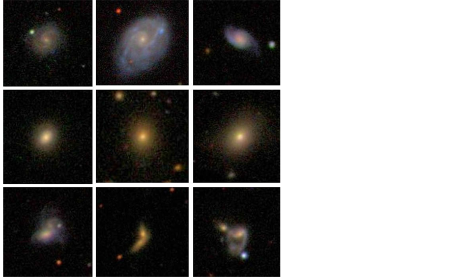
Figure 1. Sample galaxy images from the SDSS [1] .
The SDSS provides hundreds of such features for each object that are automatically measured as part of its data pipeline [2] . In selecting a subset of these features to use for classification, it is important that the features chosen characterize the categories desired. In other words, a feature must tend to have particular values for each of the categories [13] . The more diagnostic the chosen features are, the higher the resulting classification accuracy will be. Having more features though increases the computational time of the learning. Therefore, it is desirable to use a small set of features that characterizes each of the categories well. Certain subsets have been published as being useful for galaxy classifications [12] . Such published feature sets have been successfully used in many studies dealing with the classification of galaxy morphologies [8] .
Several different machine learning algorithms have been applied to this photometric data in order to automate classification. One of the most prominent examples of this is the use of neural networks. This has been one of the most successful attempts at automatic classification to date [13] . Other algorithms that have been applied to galaxy morphologies include the use of regression [14] . There has been less research with Support Vector Machines in this area [7] . This paper applies the Krylov iterative methods for the SVM algorithm to solve this classification problem.
3. Support Vector Machines
Support Vector Machines (SVMs) represent another potential method to classify galaxy morphologies. First introduced by Vapnik in 1992, the algorithm has been applied to many real world applications [15] . For example, the SVM has been utilized in bioinformatics to predict disease susceptibility [4] . It reads in sequences of genetic information, which are assigned the categories of sick and healthy, and uses it to predict an individual’s disease susceptibility. Another example where the SVM has been applied is in text classification [6] . Samples of text are analyzed and attempted to be placed into certain categories. This has several applications, such as email filtering, web searches, and product recommendations. The SVM has also been applied to astronomical data before. It has been used to distinguish between images of stars and galaxies in other sky surveys [5] .
An essential part of the SVM algorithm is how it treats its data. Each individual object must be represented in the form of a single data point. This data point consists of two pieces of information: a feature vector and a label [16] . The label indicates which category the object belongs to. A positive value indicates the first category and a negative one indicates the second category [3] . The feature vector is a numerical representation of the object. It consists of a set of values, or features, and each one of these features characterizes a certain aspect of the object. In the case of galaxy morphologies, this feature set will be the photometric parameters that describe the physical structure of the galaxy.
The SVM treats each of these data points as a point in multidimensional space. During the training phase of the algorithm, the SVM reads in a set of data points whose categories are known. The goal of the algorithm is to be able to separate the data into two groups when the dataset is plotted in space. To do this, it attempts to draw a hyperplane between the two clusters of points. In order to separate the entire feature space, the dimensionality of the hyperplane is always one less than the dimensionality of the feature vectors. For example, in a simple two dimensional problem the hyperplane is a line. In an ideal case, this hyperplane will be able to cleanly separate the two groups, with no points falling on the wrong side of the hyperplane. This is known as a linearly separable problem [15] . Each data point on one side of the hyperplane will belong to the first category, and the ones on the other side will belong to the second category.
There are infinitely many possible hyperplanes that can be drawn in order to separate the two categories. It is desirable to find the optimal hyperplane, or the one that can provide the best possible classification. This hyperplane will have the maximum possible distance between itself and the points that are closest to it. These closest points are known as the support vectors [16] . To find this hyperplane, it is necessary to solve a quadratic programming problem that maximizes the distance from the hyperplane to the support vectors. This ends up being a minimization problem that can be solved using standard mathematical techniques [5] . This can be solved using direct solvers that achieve the exact solution, or an iterative solver that approximates the solution over many iterations [3] . Direct solution methods are very expensive in both memory space and CPU time for large size problems. Once the solution is achieved, the result will provide the specifications for the optimal hyperplane. This hyperplane can then be used for prediction. Data points whose categories are not known are read in to the SVM. The category is predicted based on which side of the hyperplane the feature vector falls on.
There are many generalizations that can be made to this basic version of the SVM algorithm. One of these is to generalize the unrealistic assumption that the data is linearly separable. In most real world situations, the two categories will overlap. It will not be possible to cleanly draw a hyperplane between them [15] . To work around this problem, a slack variable is introduced that represents the amount that each data point is on the wrong side of the hyperplane [3] . This results in a slightly different quadratic programming problem that attempts to get as many points as possible on the correct side of the plane. Another generalization of the SVM is the use of separating surfaces other than the hyperplane. This is known as the kernel trick. The kernel trick maps the feature vectors from the original dataset into even higher dimensional space [5] . This is useful when the data cannot be separated easily by a linear separating surface such as the hyperplane, but can be separated in higher dimensions. This allows the use of a non-linear separating surface in the lower dimensional space. Examples of kernel functions include power functions and polynomials [3] . These series of generalizations enable the SVM algorithm to be very robust and provide high classification accuracies. A gaussian radial basis kernel was used in this paper to increase the dimensionality of the dataset and to improve classification accuracy.
4. Iterative Methods
The quadratic programming problem is the most computationally intensive part of the SVM algorithm. Any quadratic programming problem can be formulated as the solution to a system of linear equations. This be solved by using direct solvers such as Gaussian elimination in order to achieve an exact solution to the problem. However, they are often prohibitively expensive on large datasets [17] . For the Gaussian elimination method, the floating point operation count is on the order of O(N3), where N is the number of unknowns (columns) of the coefficient matrix A of the matrix equation. In contrary, the complexity of the Krylov iterative methods such as the biconjugate gradient (BiCG) type iterative methods is on the order of O(NiterN2) if the convergence is achieved in Niter iterations. Therefore, Krylov iterative methods can be applied to this problem with a much faster runtime. Such methods converge on the optimal solution over many iterations. Though these methods only provide an approximation, in most cases this approximation is close enough for classification purposes.
Krylov iterative methods are considered to be the most effective iterative solution methods currently available [18] -[20] . Krylov iterative methods are some of the most commonly used non-stationary examples of these solvers. This class of solvers relies on sets of orthonormal vectors within a Krylov subspace [20] . A basis is formed by successively multiplying the objective matrix by the residual or error of the approximation [19] . This matrix vector product accounts for the major computational cost of these algorithms. The approximation at each iteration can then be determined by minimizing the residual over this subspace. The Krylov iterative methods such as BiCG require the computation of some matrix-vector product operations at each iteration, which account for the major computational cost of this class of methods.
We conduct an experimental study on the behavior of four Krylov iterative methods, BiCG, BiCGSTAB, QMR, and GMRES. These four are some of the well-known Krylov iterative methods which are applicable to non-Hermitian matrices. The BiCG method is a generalized form of the conjugate gradient method [21] . The algorithm involves two matrix vector products, one involving the objective matrix and the conjugate transpose of the matrix. BiCG often exhibits irregular convergence behavior, and very little is known theoretically about its behavior. The biconjugate gradient stabilized (BiCGSTAB) method was developed in order to smooth the convergence by introducing a stabilizer [22] . A residual vector is minimized in this process. Similarly, the quasi minimal residual (QMR) also seeks to stabilize convergence [23] . It solves the reduced tridiagonal system in a least squares sense, and utilizes look-ahead techniques in order to avoid breakdowns. Another modern method is the generalized minimal residual method (GMRES) [24] . This method utilizes a least-squares solve and update process on the sequence of orthogonal vectors.
For symmetric positive definite systems the BiCG method delivers the same results as the conjugate gradient (CG) method, but at twice the cost per iteration. For nonsymmetric matrices it has been shown that in phases of the process where there is significant reduction of the norm of the residual, the method is often more or less comparable to full GMRES (in terms of the numbers of iterations) [23] . Finally, for comparison purposes the successive over-relaxation (SOR) method is included. The SOR is not a Krylov method; it is basic in that it is an extrapolation of the Gauss-Seidel method [25] . Hence, a total of five methods are examined in this paper.
5. Methodology
The SVM implemented for this research is a variation known as the Mangasarian-Musicant [3] . This was selected due to its brevity. A gaussian radial basis kernel was used to increase the dimensionality of the dataset and to improve classification accuracy. The resulting kernel is a completely dense matrix. The iterative methods implemented were based on the algorithms presented in [26] .
The SVM algorithm is traditionally a binary classifier, meaning that it can place objects into one of two categories. To classify galaxy morphologies in a realistic way though, it must be able to classify into the three categories of spiral, elliptical, and irregular galaxies. Though multiclass variations of the SVM exist, they are considered unreliable and do not work well with all datasets [14] . This paper implements multi-classification by using multiple classifiers in a tier structure. In this structure, a three category sample is first split using a standard binary SVM classifier. One of the three categories is chosen to be separated in this first tier. This is known as a one against all classification, in which the SVM is trained to place objects into either the chosen category or everything else. A second binary classifier is then used to separate the remaining two classes. The SVM is trained on the two classes, and a prediction is assigned to any object that was previously placed in the everything else category.
The data for this research was taken from two sources. First, the photometric data was taken from the SDSS dataset. This photometric data is automatically created by the SDSS pipeline, and is accessible via a structured query language (SQL) interface. A total of 23 different features listed in Figure 2 were chosen for use with the SVM. This feature set includes measurements of structure such as ellipticity, Petrosion flux, and the de Vacouleurs fit axis ratio as well as spectral measurements. These measurements tend to describe structural characteristics and colors of the images, as these metrics do not vary with the distance of the galaxy. These features were included several times for the i and r bandwidths of the survey, which indicate the wavelength of light in which they were captured. Previous work has found that multiple bandwidths often provide different values for the same feature, and thus can provide more information to the classifier [12] . This feature set has been found to be diagnostic for the three categories of galaxies, and was chosen due to its success in being used with previous machine learning algorithms [8] .
The second set of data required is the training data for each of the objects. The category of each object is needed to train the SVM and then determine classification accuracy. This information was taken from the Ga- laxy Zoo project [10] . This project was a citizen science effort, where over the course of several years volunteers could go to a website and manually classify images of galaxies. For each object, if users differ, the category
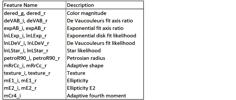
Figure 2. Photometric data feature set [5] .
receiving the most votes is the one assigned to that object. The resulting dataset was released to the public. These classifications have been found to be similar those done by professional astronomers [12] . Though biases from human classification have been shown to exist, these have been studied in detail and have been corrected [9] . The resulting dataset can therefore be used for training purposes, and has been successfully used in the past. Each object in the Galaxy Zoo dataset corresponds to an object in the SDSS, and so the two datasets can be correlated to create a master set with classification information.
The Galaxy Zoo dataset provides the percent of votes that each category received. For training the SVM, only objects receiving more than 80% in one category were chosen to reduce noise in the dataset [10] . Objects assigned to the spiral category for training contained the categories of clockwise spiral, anti-clockwise spiral, and edge-spiral from the Galaxy Zoo dataset. Objects assigned to the irregular category were taken from the category of merge from the Galaxy Zoo dataset.
6. Numerical Results
A total of eleven experiments were run. Five data samples were used for each one of these. Each training sample contained 3000 galaxies, with 1000 objects from each category. A separate testing sample for each of the train- ing samples was used to determine the classification accuracy. These testing samples also contained 3000 ob- jects.
Experiments 1 through 6 utilized the basic SOR solver to measure a baseline performance of the SVM with differing galaxy categories. The first three experiments measured the ability of the SVM to distinguish between each pair of categories. The accuracy of the SVM was measured on the categories of spiral and elliptical, spiral and irregular, and elliptical and irregular in Experiments 1, 2, and 3, respectively (see Table 1). The second set of three experiments measured the accuracy of the three class SVM (see Table 2). A separate run was carried out for each of the three categories as the first tier, or the category that was split first. Experiment 4 separated the spiral category first, Experiment 5 separated ellipticals first, and Experiment 6 separated irregulars first (see Tables 3-5). The accuracy was measured for each of the experiments. The metrics include the accuracy, which is a simple measure of the number of the objects correctly classified divided by the total number of objects. The sensitivity is the proportion of objects in the positive category that are correctly classified as such. The specific- ity is the proportion of objects in the negative category that are correctly classified. The number of iterations each solver took to converge and the solving time are also included. For Experiments 7 through 11, each of the iterative solvers was used to solve the quadratic programming problem within the SVM, and the resulting solu- tion used for classification (see Table 7). Five data samples were used for each solver. For these experiments, only the spiral and elliptical categories were chosen in order to compare the efficiencies of the solvers.
The results of Experiments 1-3 are presented in Table 1. The table summarizes the average accuracies and runtimes of the five samples in each two class separation. The accuracy between each of the two categories was

Table 1. Averages of two class SVM: Experiments 1-3.
Table 2. Averages of three class SVM: Experiments 4-6.
Table 3. Experiment 4: Confusion matrix, spiral first tier.
Table 4. Experiment 5: Confusion matrix, elliptical first tier.
Table 5. Experiment 6: Confusion matrix, irregular first tier.
comparable to those achieved by other classification methods, such as the use of neural networks [5] . Out of the three combinations, the SVM was able to distinguish between spirals and ellipticals at the highest accuracy of 96.8%. This was followed by ellipticals and irregulars with an accuracy of 88.5%. The SVM was the least accurate in classifying spirals and irregulars, having an accuracy of 71.6%. The SVM was more easily able to distinguish ellipticals than the other categories. This suggests that elliptical galaxies, with their featureless disks, are much easier to characterize in the feature set. The sensitivity and specificity did not differ significantly in the first two experiments. This signifies that the classification did not tend to classify one category more aggressively than the other. When classifying elliptical and irregular galaxies, however, the specificity was slightly higher than the sensitivity. This signifies that the classification tended to lean in the direction of irregular galaxies.
Also of note is the run time for these experiments. The spiral and elliptical classification required the least average runtime of 4.0 seconds with an average of 123 iterations. However, the longest runtime of 10.6 seconds for the spiral and irregular classification required the least number of iterations at 118. There is no clear correlation between runtime and iteration count. This is due to the differing time per iteration for each of the convergences. There was a correlation though between the run times and the accuracy of the classification. Lower classification accuracy corresponded with a higher runtime. The least accurate classification between spiral and irregular had the highest runtime.
The summary results from the three different implementations of the three class SVM in Experiments 4-6 are presented in Table 2. The overall accuracy is presented as well as the percentage correctly classified for each of the three categories. Separating the spiral category and elliptical category first both resulted in comparable performance in terms of accuracy. The total percent of objects correctly classified for the spiral and elliptical first tier was 73.1% and 74.3% respectively. Separating the irregular galaxies first resulted in a noticeable decrease in accuracy to 67.2%, though it still provided a useful accuracy. The primary reason for this can be seen in the noticeable drop in percent of irregulars correctly classified to 37.7%. This demonstrates that the SVM has difficulty in performing a one against all classification with irregulars. This suggests the broad range of feature values of the irregular galaxy are difficult to distinguish between the two other categories.
All three multi-classifications implementations resulted in very high accuracies for the elliptical category. This further shows the ability of the SVM to distinguish this category from the others. The spiral category also achieved percentages as high as 81.0%, though this is noticeable lower than the elliptical category. The irregular category contained the lowest percentages out of the three. In terms of time, the elliptical first tiers resulted in the most efficient solving with a time of 23.1 seconds. The spiral first tier took the most time at 45.5 seconds.
Confusion matrices are also presented for the three class SVM’s in Tables 3-5. Each row corresponds to the actual category of galaxy and each column corresponds to the predicted category, or the category that the object was classified into. This shows for each of the actual categories what objects tended to be classified as and where the error in classification is occurring. In each of the three tables, it is clear that spiral galaxies tend to be confused most with irregular galaxies. As much as 32.1% of spiral galaxies are classified as irregular. It is rare that a spiral galaxy is classified as elliptical, as this percentage tended to be low. Irregular galaxies, however, are classified as elliptical frequently, with rates as high as 19%. Overall, the most spread in classification can be seen in the irregulars, reflecting the greater amount of error in classification for this category.
Receiver Operating Characteristic (ROC) graphs are presented in Figures 3-6. The ROC curve plots the tradeoff between the true positive (TP) and false positive (FP) classification rate. ROC curves are traditionally used with probabilistic classifiers. The SVM is a deterministic classifier, meaning it assigns a definite category to its prediction. However, it is possible to apply ROC graphs to the SVM by comparing the threshold values to internally computed scores. Figure 3 displays three separate curves for the two class experiments. In this case,
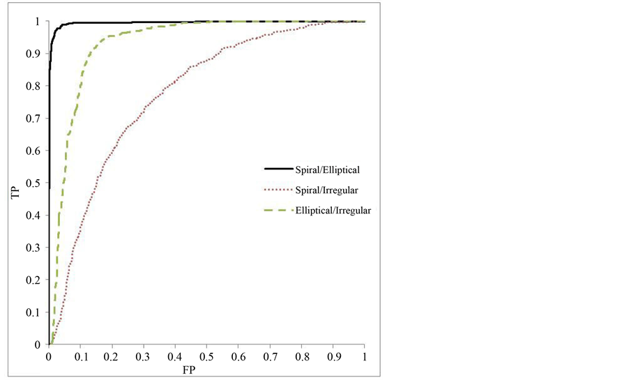
Figure 3. Experiments 1-3 ROC curve.
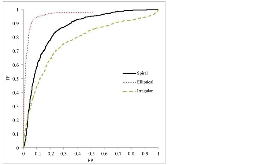
Figure 4. Experiment 4: ROC curve, spiral first tier.
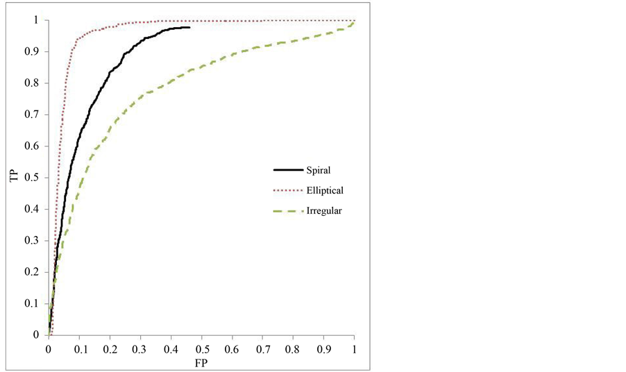
Figure 5. Experiment 5: ROC curve, elliptical first tier.
the positive category is arbitrarily chosen between the two. The higher accuracy of the classification spiral and elliptical categories can be seen as the curve approaches perfect classification at the point (0, 1), corresponding to classifying all true positives with no false positives. The area under the curve (AUC) for each of the three curves is presented in Table 6. These numbers provide an overall summary of its performance across all threshold values. It also represents statistically the probability that the classifier will rank a given positive instance
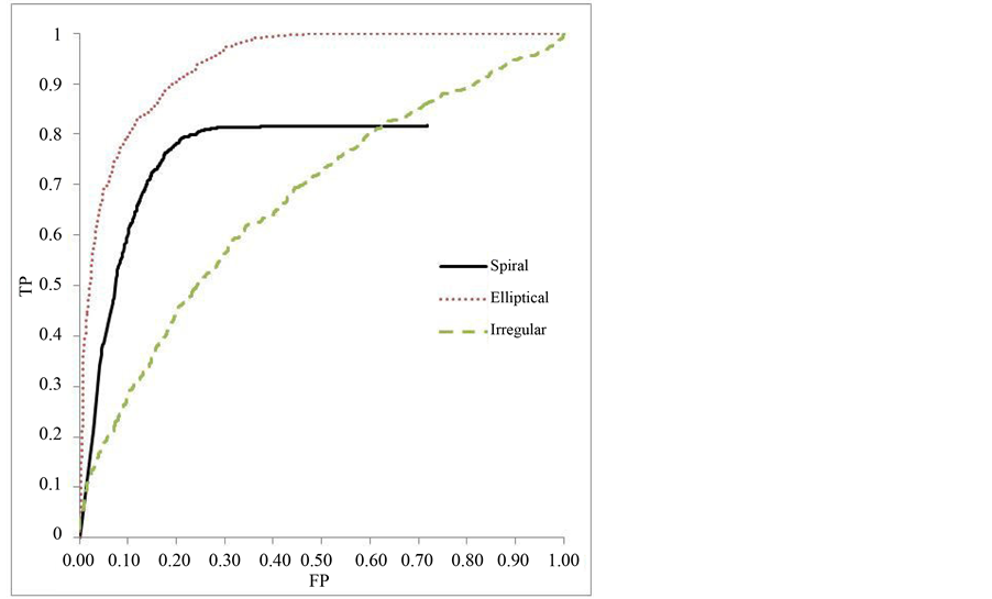
Figure 6. Experiment 6: ROC curve, irregular first tier.
higher than a given negative instance [27] .
Figures 4-6 demonstrate the performance of the three class classifier. A true ROC curve for three classes would mark the tradeoff between true positive and false positive for each of the three categories resulting in a six dimensional curve. To simplify understanding, the class reference formulation of a three class ROC is pre- sented [27] . The class reference formulation plots a curve for each of the classes. Each of the classes is treated as the positive instance and the others as negative for the single curve. These curves also show the performance of the classifier over a varying threshold value. However, the behavior differs slightly due to the tiered classifica- tion and the use of two classifiers. Each of the SVMs will have a threshold value applied. As a result, the true positive and false positive rate may not reach a value of one.
The results for Experiments 7 through 11 are presented in Table 7. These are the average results for each of the Krylov iterative solvers in addition to SOR as a comparison. All solvers were able to successfully converge on a solution. Of note is the difference in the sensitivity and specificity in these results. In each of the solvers, the sensitivity was much higher (approximately 98%) than the specificity (approximately 42%). This demon- strates that the SVM was much more aggressive in classifying spirals than ellipticals. As a result, the spiral was classified at a higher rate. When comparing the solvers, all five achieved similar accuracies. In fact, the four Krylov methods, BiCG, BiCGSTAB, QMR, and GMRES, all achieved the same solution with each of the data samples. This is to be expected, as the methods should converge on the same solution.
The runtimes and iteration counts, however, did differ significantly. Out of the four Krylov iterative methods, GMRES was clearly the most efficient, achieving the lowest runtime of 2.0 seconds. It also had the least number of iterations at 53. Following GMRES, BiCGSTAB and QMR had similar runtimes of 4.7 seconds and 4.8 seconds respectively. Their iteration counts were also similar in these methods. The slowest of the Krylov itera- tive methods was the BiCG with a runtime of 6.1 seconds and an iteration count of 93. With these methods, there is a clear correlation between runtime and the number of iterations. Higher runtimes corresponded to high- er numbers of iterations. This suggests that the time per iteration was relatively similar for these four methods. All these methods outperformed the SOR by a large margin. The time was significantly higher at 16.1 seconds.
Convergence histories are presented in Figures 7-10. These histories show the change in the residual norm as the iterations converge to the solution. In all the methods, the residual dropped rapidly from its initial position, and spent the majority of its iterations slowly approaching its solution at 0. Most noteworthy in these histories is
Table 6. ROC AUC Experiments 1-3.
Table 7. Experiments 7-11: Averages of iterative solvers.
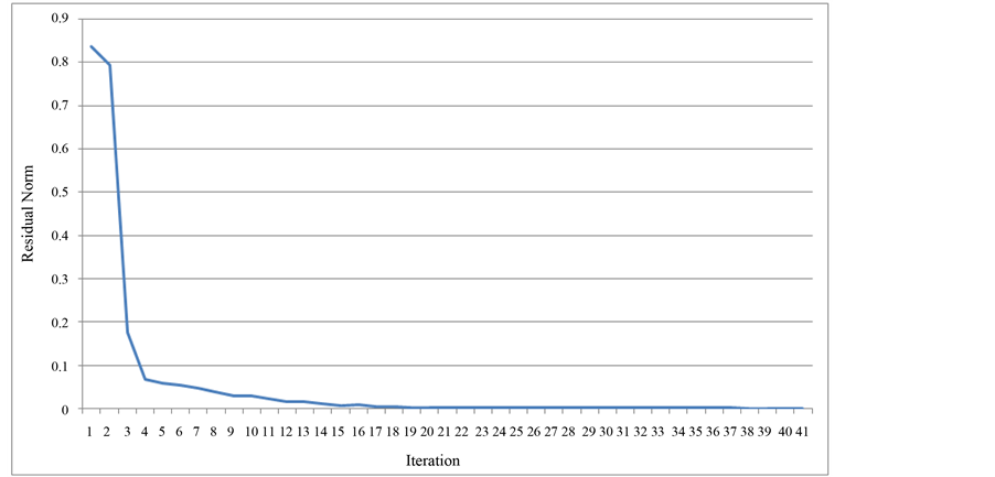
Figure 7. Convergence history of BiCGSTAB solver.
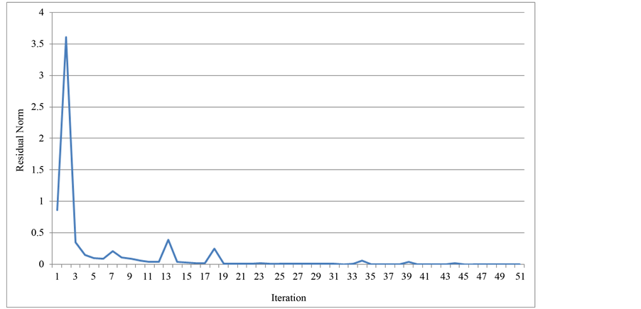
Figure 8. Convergence history of BiCG solver.
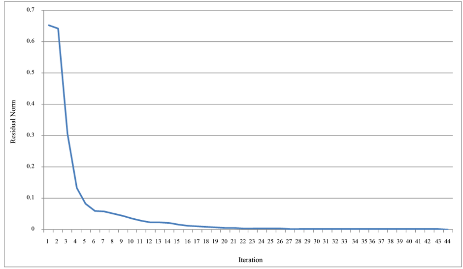
Figure 9. Convergence history of QMR solver.
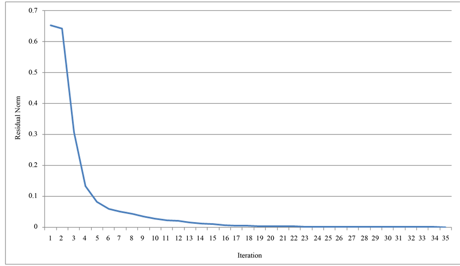
Figure 10. Convergence history of GMRES solver.
the BiCG. The erratic behavior of the iterative method is displayed in the many times that the residual norm rises before it drops again. Few theoretical results are known about the convergence of BiCG [17] [19] [26] . In practice, it is observed that the convergence behavior may be quite irregular, and the method may even break down. The breakdown situation due to the possible event by the so-called a look-ahead strategy [28] . The other breakdown situation occurs when the lower upper (LU) decomposition fails, and can be repaired by using another decomposition. Sometimes, the breakdown or near-breakdown situations can be satisfactorily avoided by a restart at the iteration step immediately before the (near-)breakdown step. The stabilizing effect of the BiCGSTAB can be seen in its smoother convergence. This resulted in BiCGSTAB having a lower runtime than the BiCG. Another possibility is to switch to a more robust method, like GMRES [20] [26] .
7. Conclusions
Support Vector Machines (SVMs) can be applied confidently to the problem of classifying galaxy morphologies. As modern sky surveys continue to produce more and more data, machine learning algorithms such as the SVM will be required to analyze the data. The presented algorithm can be feasibly used to classify the entire SDSS dataset. The automation of the galaxy classification process will save countless hours that are required to manually classify objects. Astronomers will be able to make use of the addition of this information to these catalogues of galaxies to test many theories about the universe and gain a better understanding about the evolution of galaxies.
The numerical results demonstrate the high accuracy of classification by the SVM. The results of two-class separation between the spiral and elliptical categories are particularly noteworthy. The SVM also provides useful accuracies on a three-class sample. In a real world application, this would be the most likely use of the SVM, as sky surveys would contain all three classes. The implementation of the multi-classification SVM can have an effect on the accuracy of the classification. The results may assist researchers in selecting a first tier for separation. Both the spiral and elliptical categories provide comparable accuracy as the first tier. However, the runtime for the elliptical tier is significantly smaller. This suggests that the elliptical first tier would be the most useful implementation of a three-class SVM.
The results also demonstrate the challenge of using classification algorithms on the irregular category of galaxies. In the two-class separation, it was much harder for the SVM to distinguish between the irregular and the other two categories. This is also demonstrated in the low accuracy of the one against all classification in the irregular first tier. This is a challenge related to the definition of irregular galaxies. As the category contains galaxies with no definite structure that do not meet the requirements of either of the other categories, it is difficult to characterize the category within the feature set, and it is less diagnostic. The values of the feature measurements tend to vary greatly from object to object. It is therefore frequently confused with other objects. The featureless disk of elliptical galaxies, by contrast, is relatively easy to characterize in a feature set. It is therefore easier to separate in classification. Spiral galaxies also have a definite structure in the form of spiral arms that can be used for classification. One of the challenges with this category is ensuring that it is not confused with irregular galaxies.
The comparison of the iterative solvers may assist researchers in selecting an efficient method to solve the quadratic programming problem within the SVM algorithm. In all cases, Krylov iterative methods performed more efficiently than the basic SOR method while achieving almost identical classification accuracies. Their robust algorithms allow them to solve many real world applications with a fast runtime. The results suggest that the GMRES iterative method is the most useful method to use for classifying galaxy morphologies. It has the fastest runtime of all the methods.
Future work in this area can attempt to increase the classification accuracy of the SVM. One of the greatest sources of error in classification is the irregular category. Improving this accuracy would greatly improve the overall accuracy. A potential way to do this might involve finding a feature set that better characterizes the category. Further research could focus on further improving the runtime of the algorithm. Techniques such as preconditioning can be used to decrease the number of iterations of the solvers.
Cite this paper
MatthewFreed,JeonghwaLee, (2015) Krylov Iterative Methods for Support Vector Machines to Classify Galaxy Morphologies. Journal of Data Analysis and Information Processing,03,72-86. doi: 10.4236/jdaip.2015.33009
References
- 1. Szalay, A., et al. (2000) Designing and Mining Multi-Terabyte Astronomy Archives: The Sloan Digital Sky Survey. Proceedings of the 2000 ACM SIGMOD International Conference on Management of Data, 451-462.
http://dx.doi.org/10.1145/342009.335439 - 2. Abazajian, K.N. (2009) The Seventh Data Release of the Sloan Digital Sky Survey. Astrophysical Journal Supplement Series, 182, 543-558.
http://dx.doi.org/10.1088/0067-0049/182/2/543 - 3. Press, W.H., et al. (2007) Numerical Recipes: The Art of Scientific Computing. Cambridge University Press, Cambridge.
- 4. Freed, M., Collins, J. and Lee, J. (2011) Training Support Vector Machine Using Adaptive Clustering. Proceedings of the International Conference on Bioinformatics and Computational Biology, 131-135.
- 5. Fung, G. and Mangasarian, O. (2000) Data Selection for Support Vector Machine Classifiers. Proceedings of the 6th ACM SIGKDD International Conference on Knowledge Discovery and Data Mining, 64-70.
http://dx.doi.org/10.1145/347090.347105 - 6. Tong, S. and Koller, D. (2002) Support Vector Machine Active Learning with Applications to Text Classification. The Journal of Machine Learning Research, 2, 45-66.
- 7. Freed, M. and Lee, J. (2013) Application of Support Vector Machines to the Classification of Galaxy Morphologies. Proceedings of the International Conference on Computational and Information Sciences, Shiyang, 21-23 June 2013, 322-325.
http://dx.doi.org/10.1109/iccis.2013.92 - 8. Gauci, A., et al. (2010) Machine Learning for Galaxy Morphology Classification. Monthly Notices of the Royal Astronomical Society.
- 9. Bamford, S.P., et al. (2008) Galaxy Zoo: The Dependence of Morphology and Colour on Environment. Monthly Notices of the Royal Astronomical Society, 393, 1324-1352.
http://dx.doi.org/10.1111/j.1365-2966.2008.14252.x - 10. Lintott, C., et al. (2008) Galaxy Zoo: Morphologies Derived from Visual Inspection of Galaxies from the Sloan Digital Sky Survey. Monthly Notices of the Royal Astronomical Society, 383, 1179-1189.
http://dx.doi.org/10.1111/j.1365-2966.2008.13689.x - 11. Shamir, L. (2009) Automatic Morphological Classification of Galaxy Images. Monthly Notices of the Royal Astronomical Society, 349, 1367-1372.
http://dx.doi.org/10.1111/j.1365-2966.2009.15366.x - 12. Banerji, M., Lahav, O., Lintott, C.J., Abdalla, F.B., Schawinski, K., Bamford, S.P., et al. (2010) Galaxy Zoo: Reproducing Galaxy Morphologies via Machine Learning. Monthly Notices of the Royal Astronomical Society, 406, 342-353.
http://dx.doi.org/10.1111/j.1365-2966.2010.16713.x - 13. Calleja, J. and Fuentes, O. (2004) Machine Learning and Image Analysis for Morphological Galaxy Classification. Monthly Notices of the Royal Astronomical Society, 349, 87-93.
http://dx.doi.org/10.1111/j.1365-2966.2004.07442.x - 14. Anderson, B., Moore, A., Connolly, A. and Nichol, R. (2004) Fast Nonlinear Regression via Eigenimages Applied to Galactic Morphology. Proceedings of the 10th ACM SIGKDD International Conference on Knowledge Discovery and Data Mining, Seattle, 22-25 August 2004, 40-48.
http://dx.doi.org/10.1145/1014052.1014060 - 15. Cortest, C. and Vapnik, V. (1995) Support-Vector Machines. Machine Learning, 20, 273-297.
http://dx.doi.org/10.1007/BF00994018 - 16. Bennet, K. and Demiriz, A. (1998) Semi-Supervised Support Vector Machines. Proceedings of Neural Information Processing Systems.
- 17. Lee, J., Zhang, J. and Lu, C. (2003) Performance of Preconditioned Krylov Iterative Methods for Solving Hybrid Integral Equations in Electromagnetics. Journal of Applied Computational Electromagnetics Society, 18, 54-61.
- 18. Axelsson, O. (1994) Iterative Solution Methods. Cambridge University Press, Cambridge.
http://dx.doi.org/10.1017/CBO9780511624100 - 19. Greenbaum, A. (1997) Iterative Methods for Solving Linear Systems. Society for Industrial and Applied Mathematics.
http://dx.doi.org/10.1137/1.9781611970937 - 20. Saad, Y. (2003) Iterative Methods for Sparse Linear Systems. Society for Industrial and Applied Mathematics.
http://dx.doi.org/10.1137/1.9780898718003 - 21. Lanczos, C. (1952) Solution of Systems of Linear Equations by Minimized Iterations. Journal of Research of the National Bureau of Standards, 49, 33-53.
http://dx.doi.org/10.6028/jres.049.006 - 22. van der Vorst, H. (1992) Bi-CGSTAB: A Fast and Smoothly Converging Variant of Bi-CG for the Solution of Non-symmetric Linear Systems. SIAM Journal on Scientific and Statistical Computing, 13, 631-644.
http://dx.doi.org/10.1137/0913035 - 23. Freund, R. and Nachtigal, N. (1991) QMR: A Quasi-Minimal Residual Method for Non-Hermitian Linear Systems. Numerische Mathematik, 60, 315-339.
http://dx.doi.org/10.1007/bf01385726 - 24. Saad, Y. and Schultz, M. (1986) GMRES: A Generalized Minimal Residual Algorithm for Solving Nonsymmetric Linear Systems. SIAM Journal on Scientific and Statistical Computing, 7, 856-869.
http://dx.doi.org/10.1137/0907058 - 25. Kahan, W. (1958) Gauss-Seidel Methods of Solving Large Systems of Linear Equations. PhD Thesis, University of Toronto, Toronto.
- 26. Barrett, R., Berry, M., Chan, T.F., Demmel, J., Donato, J., Dongarra, J., et al. (1994) Templates for the Solution of Linear Systems: Building Blocks for Iterative Methods. 2nd Edition, Society for Industrial and Applied Mathematics, Philadelphia.
http://dx.doi.org/10.1137/1.9781611971538 - 27. Fawcett, T. (2003) Roc Graphs: Notes and Practical Considerations for Data Mining Researchers. HP Laboratories.
- 28. Parlett, B.N., Taylor, D.R. and Liu, Z.A. (1985) A Look-Ahead Lanczos Algorithm for Unsymmetric Matrices. Mathematics of Computation, 44, 105-124.
http://dx.doi.org/10.2307/2007796
NOTES

*Corresponding author.