International Journal of Geosciences
Vol. 4 No. 2 (2013) , Article ID: 29301 , 15 pages DOI:10.4236/ijg.2013.42031
Similarity Measures of Satellite Images Using an Adaptive Feature Contrast Model
1State Key Laboratory of Earth Surface Processes and Resource Ecology, Beijing Normal University, Beijing, China
2Key Laboratory of Mine Spatial Information Technologies, State Bureau of Surveying and Mapping, Beijing, China
3CNPC Research Institute of Safety & Environment Technology, Beijing, China
Email: *hongtang@bnu.edu.cn
Received November 9, 2012; revised December 8, 2012; accepted January 12, 2013
Keywords: Similarity Measurement; Feature Contrast Model; Set-Theoretic Similarity; Image Retrieval
ABSTRACT
Similarity measurement is one of key operations to retrieve “desired” images from an image database. As a famous psychological similarity measure approach, the Feature Contrast (FC) model is defined as a linear combination of both common and distinct features. In this paper, an adaptive feature contrast (AdaFC) model is proposed to measure similarity between satellite images for image retrieval. In the AdaFC, an adaptive function is used to model a variable role of distinct features in the similarity measurement. Specifically, given some distinct features in a satellite image, e.g., a COAST image, they might play a significant role when the image is compared with an image including different semantics, e.g., a SEA image, and might be trivial when it is compared with a third image including same semantics, e.g., another COAST image. Experimental results on satellite images show that the proposed model can consistently improve similarity retrieval effectiveness of satellite images including multiple geo-objects, for example COAST images.
1. Introduction
The effectiveness of retrieving images from a large Remote-Sensing (RS) archive weightily relies on the description of images [1,2]. Low-level visual features, e.g., color, texture and shape, are widely used in image retrieval systems, since they are easy to extract [3]. It is well known that there exists an evident semantic gap between the demanding of users and the representation of low-level features [4]. Therefore, it seems more attractive to represent images using high-level semantic features. Much attention has been paid to derive semantic features from low-level features [5-9] or bridge the gap through interaction between users and retrieval systems [10-13]. When multiple semantic features are available, cooccurrence semantic features are often employed to measure similarity between images [3,8,11,14]. Little attention has been explicitly paid to various distinctions of available semantics, when the semantic features are employed to measure the similarity. The possible reason is that one might be more interested in whether the semantics are the same or how often the same semantics simultaneously occur in the two images. Given a set of binary semantic features for objects, Tversky argued that similarity measurements should increase with the saliency of common features (which are shared by two objects) and decrease with that of distinct features (which belong to only one of the two objects) [15-17]. As a real implementation of Tversky’s set theoretic similarity, Feature Contrast (FC) model reduces the saliency of a feature set into the sum of number of features in the feature set. The potential assumption is that features are independent and at the same level of saliency in terms of contribution to similarity measurements. As shown in Tversky’s experiments, the assumption seems reasonable when one could carefully list all necessary features to avoid or eliminate the different generality of features.
However, the above-mentioned assumption is not same as what we could expect in image retrieval. On the one hand, one still is very restricted to directly access semantic features of images. Most approaches to semantic features are to model an image as an intermediate representation through supervised or unsupervised learning, such as semantic modeling [6,8], bag of features [18-21] and probabilistic topic models [2,22]. The intermediate representation is based on models of semantics, which are either low-level visual features or text semantics [23]. In particular, when the semantics are modeled through unsupervised learning, one might have no direct access to what semantics the representations really are. Therefore, the distinction between various semantics would often be different, even if each semantic exactly corresponds to one kind of images or image parts.
On the other hand, it is intrinsic for some semantics to be at the different level of generality in satellite images. For example, term land is more general than terms island and building-area when they are relative to term water. From the viewpoint of dissimilarity, the salience of distinction between terms island and building-area is less evident than that between terms land and water. In terms of similarity measurements, the later would cause the measurement decrease more than the former. Moreover, the meaning of land would be intrinsic in the term island or building-area, when they are relative to term water. Therefore, even if term land does not appear in a list of available semantic features, it still works when terms island or building-area in the list.
In this paper, we explored similarity measures using both common and distinct features under the assumption that we have access to semantic features in a very restricted way. Specifically, semantic features are assumed to be encoded in cluster labels of regions in images. Following Tversky’s set-theoretic similarity, similarity measurements between images would increase with how many labels are common, and decrease with how many labels are distinct. In this case, we argue that the role of distinct features could change with the feature sets in comparison, since semantic features might be not at a same level of generality. Accordingly, it is necessary to regulate the saliency or role of distinct features in the similarity measurement.
The rest of this paper is organized as follows. In Section 2, two kinds of image representations used in this paper are introduced, and the limitations of Tversky’s set-theoretic similarity are outlined. To address the limitations, an extended model is presented in Section 3. Experimental results and discussions are given in Section 4. Some conclusions are drawn in Section 5.
2. Similarity Measures
Image similarity measures rest on two basic elements: finding a set of features which adequately encodes the characteristics that one intends to measure and endowing the feature space with a suitable metric [16]. One kind of similarity measure is feature vectors coupled with a geometric distance, where each dimension corresponds to a particular global attribute for instances. Another kind of similarity measure is to matching features in two sets [15]. For instance, images are represented as feature sets in the extended model, where the sets might vary in cardinality and elements lack a meaningful ordering. Then, feature matching between sets might be employed to measure image similarity. For the sake of comparison, the two kinds of similarity measures used in our experiments are represented in the following.
2.1. Image Representation
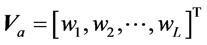
Two kinds of image representations used in this paper are illustrated in Figure 1. Firstly, each image is partitioned into regions with size of 64 × 64 pixels. Secondly, lowlevel visual features are extracted from each region. Then, all regions in the image database are clustered into L classes using the low-level features, and a digital label is allocated to each region by the clustering algorithm. At last, an image is represented as either a label vector or a set of labels.
Given image a with m regions, a set of low-level feature vectors are given by
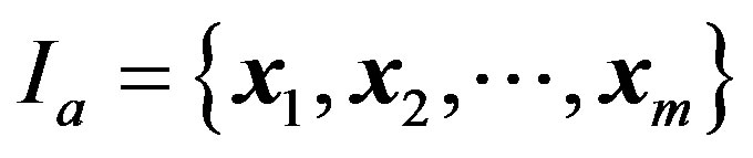 , (1)
, (1)
and image a can be represented as a feature set
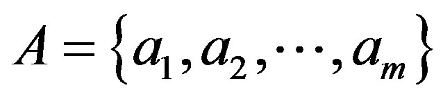 , (2)
, (2)
where 
 is one cluster of L labels from clustering using low-level features [24]. Another approach to image representation is to reconstruct a vector space using intermediate-level cluster labels of regions, for instance, Concept-Occurrence Vector (COV) used in [8]. Therefore, the COV can be written as
 (3)
(3)
where 
 might be the frequency or area percentage of regions in an image belonging to ith class. Then, general geometric distance can be used to measure similarity using COVs of images. Please note that the labels used in [8] are obtained through supervised learning. Although a supervised learning algorithm could be used learn semantic concepts more reliably, it needs intensive human annotation and is not scalable [6]. In this paper, unsupervised learning is employed to construct COV, and Kullback-Leibler divergence is used to measure image dissimilarity between two COVs.
2.2. Non-Metric Similarity
In the society of psychology, human assessment of similarity has been an active research topic for many years, since it is one of foundational cognitive problems. As outlined by [25], there exist four kinds of main approaches to similarity measures: feature-theoretic [15], geometric [26], alignment-based [27] and transformational [28]. Among these approaches, the geometric model, e.g., Minkowski-type geometric distances, is widely used in real applications. However, some psychologists argue that human similarity judgment is not a metric [15,27,28]. Many psychological approaches to nonmetric similarity are utilized to analyze or measure similarity between images. The latent reasons might consist
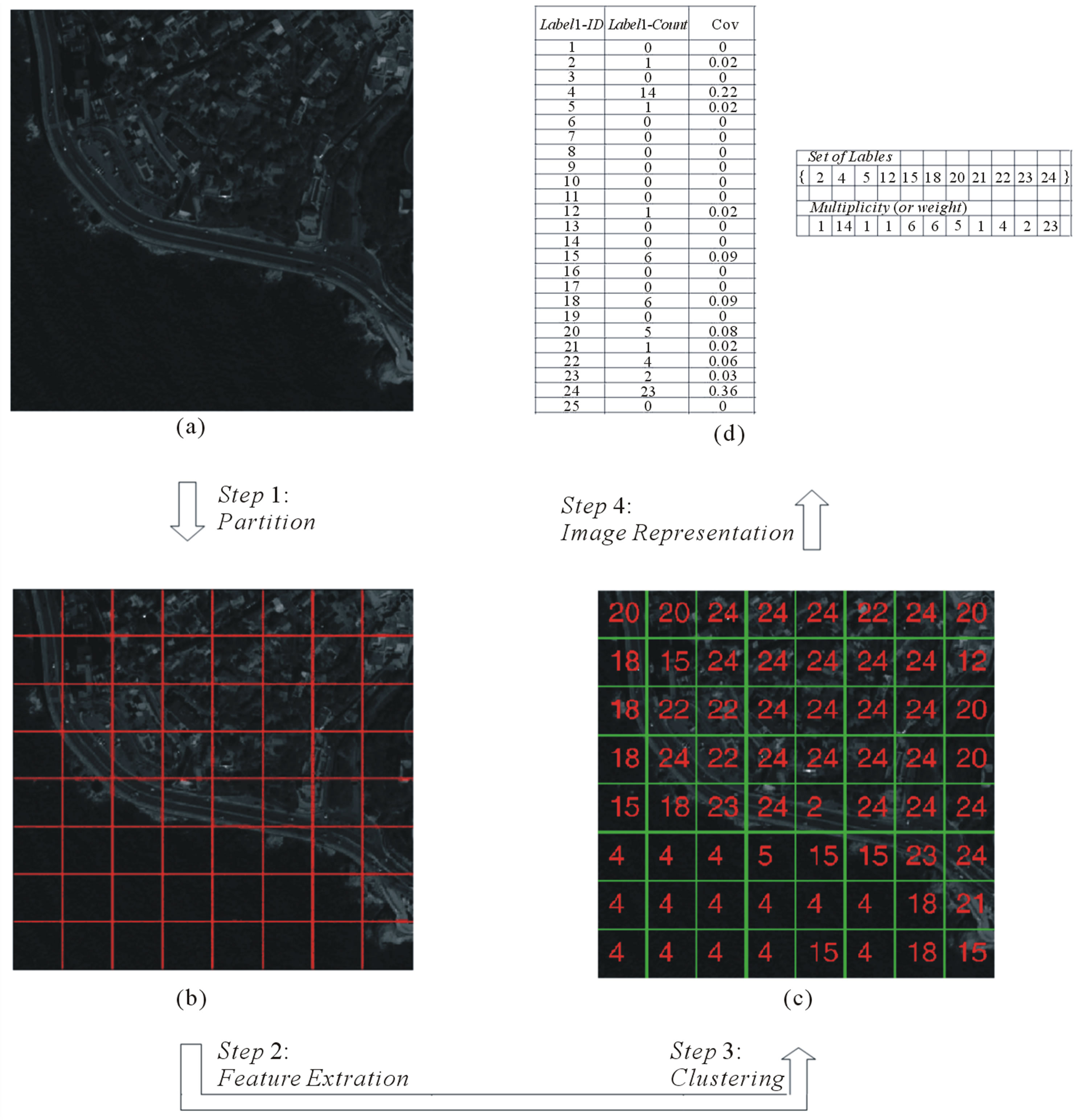
Figure 1. Image representation through label allocation. (a) Images; (b) Partitioned regions; (c) Allocated labels; (d) Vector vs. set.
in: 1) Human similarity assessment in the nature might be non-metric; 2) Those Minkowski-type geometric distances are often not good enough to characterize the similarity between images. In the rest of this section, we confine ourselves to review the FC model and its fuzzy extensions for measuring image similarity.
2.2.1. The Feature Contrast (FC) Model
Tversky challenged the dimensional and metric assumption, which underlies the geometric similarity models, and developed an alternative feature matching approach to the analysis of similarity relations [15]. The FC model is a representation form of feature matching functions, which satisfies Tversky’s assumptions of feature matching processing. Let A, B, C be the feature sets of objects a, b and c, respectively.  is a similarity measure between objects a and b. Tversky postulated five assumptions for his similarity theory, i.e., matching, monotonicity and independence, solvability and invariance [15]. Any function, which satisfies the first two assumptions, is called a matching function
 :
:
1) Matching: . That is to say that the similarity measure could be expressed as a function of three parameters: common features, which are shared by two objects (i.e.,
 ) and distinct features, which belong to only one of the two objects (i.e.,
  and
and ).
).
2) Monotonicity: 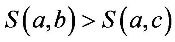 wherever
  ,
,  and
and . That implies the similarity would increase with the number of common features and decrease with that of distinct features.
As a simple form of matching function, the FC is given by
 (4)
(4)
where  is a nonnegative salience function of feature
 ; nonnegative constants
 ,
, ![]() and
and  reflect the relative salience of common features (i.e.,
 ) and two kinds of distinct feature (i.e.,
  and
and ), respectively. However, please note that the nonnegative constants do not depend on the two feature sets in comparision, i.e.,
  and
and . In addition, the salience function
  is assumed to satisfy feature additivity
 (5)
(5)
when  and
and 
 .
.
2.2.2. The Fuzzy Feature Contrast (FFC) Model
Let  be a set and
 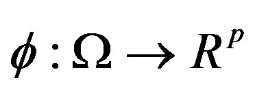 a set of p measurements on the elements of
 . Let
. Let  be a predicate about the element
 . The truth-value of the predicate
  is
is 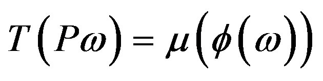 with
with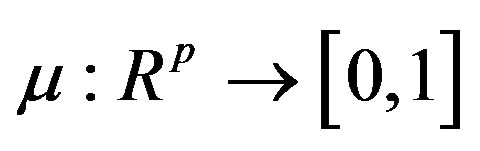 . All measurements can be collected into a vector
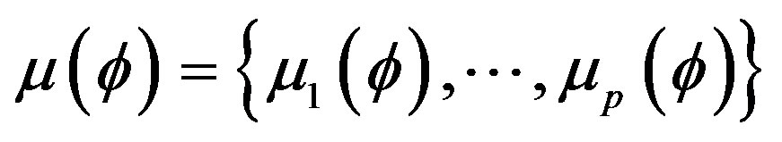 (6)
(6)
where  is the fuzzy set of p true predicates on the measurements
 [1]. Let
![]() and
and be the measurements of two objects a and b, respectively. In order to extend the FC to the fuzzy set
 , the salience function
 is given by Equation (5). The similarity measurement of the FFC model is given by
 (7)
(7)
where the intersection and difference of two fuzzy sets are respectively given by
 (8)
(8)
and
 (9)
(9)
2.3. The Limitation of the FC Model
In Tversky’s original paper, two primary comments are made about the feature representation before the theory was presented [15,17]. First, one has access to a general database of properties concerning a specific object (e.g., person or country), where the properties are deduced from human general and prior knowledge of the world. Given a specified task (e.g., identification or similarity assessment), one can extract or compile a limited list of relevant features from the database, to fulfill the requested task. Second, features are often represented as binary values, i.e., presence or absence of a specified property. The underlying assumption of the comments is that the process of feature extraction is out of similarity measures since all relevant features have been available in a suitable form (e.g., binary value) before similarity is measured. It is in the case that it seems reasonable for features to be additive in Tversky’s experiments, because the extraction or compiling of relevant features is strictly under control.
The two underlying assumptions of the feature additivity shown in Equation (5) include: 1) features are independent of each other; 2) each feature is at the same level of saliency in terms of contribution to the similarity measure. Actually, each feature is regarded as an elementary atom in the sense that it cannot be split into “finer” features any more and any object under investigation cannot be represented by two different subsets of features in an equivalent way. It is the very reason that the salience of features can be reduced to the number of features in Tversky’s experiments. The underlying assumption is that any semantic feature must not be a summary of other semantic features. According to the assumption, terms land, island and building-area should not occur in a same list of elementary features, since term land might be a summary of terms island and building-area in some senses. However, even when available semantic features themselves are well defined in the feature list to be used, the case could be still inevitable in image retrieval, because it is natural to replace some more general semantics with some specific ones when one would like to tolerate the distinction between them.
An intuitional example is shown in Figure 2, where four images (i.e., a, b, c and d) belong to three image categories: SEA, COAST and CITY. Note that the name of image category (e.g., SEA) does not denote any semantic feature but a set of images in our ground truth database. In contrast, the texts on images are desirable semantic features for corresponding image parts, such as water, island and so on. Note that these semantic features are not available in our experiments and we expect they could be encoded by cluster labels of regions during clustering. However, in current example, we suppose they are ready to use. For example, the semantic feature sets of images a, b, c and d are A = {water}, B = {water, island}, C = {water, building-area}, and D = {building-area}, respectively.
In both images b and c, there are two salient and heterogeneous objects, i.e., “sea” and “land”, which are related to a same concept “COAST”. So, most people might think that the two images b and c would be the most similar among the four images shown in Figure 2. However, this kind of human similarity judgment can not be validated by similarity measures based on the FC model. As shown in Table 1, the similarity measurement between images b and c (i.e., ) would be never higher than that between images a and b (i.e.,
 ), and that between images c and d (i.e.,
 ) at the same time. In other words, human similarity judgments
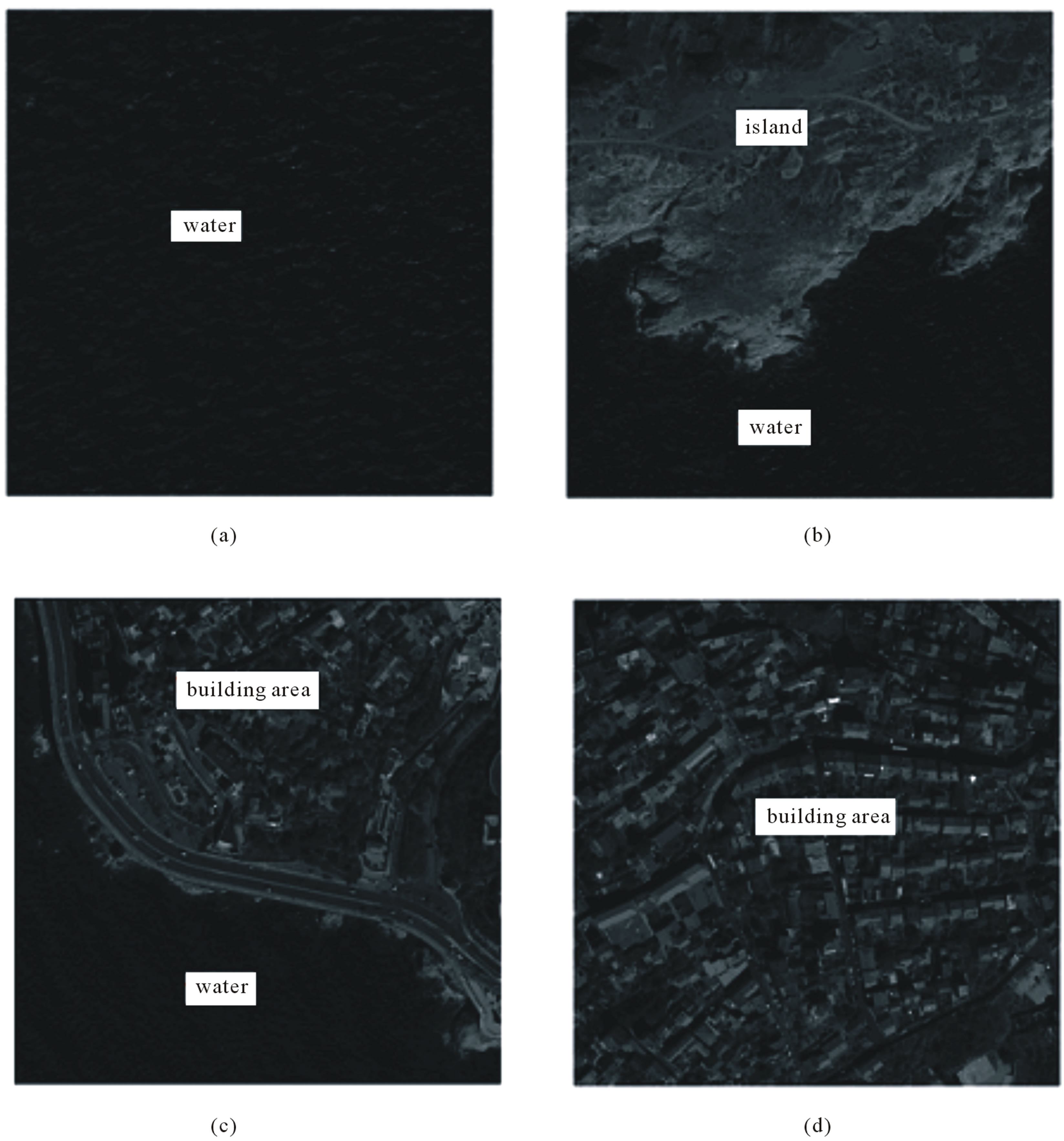
Figure 2. Example images and real semantics of regions. (a) Sea; (b) Coast; (c) Coast; (d) City.
Table 1. Similarity measurements using FC.
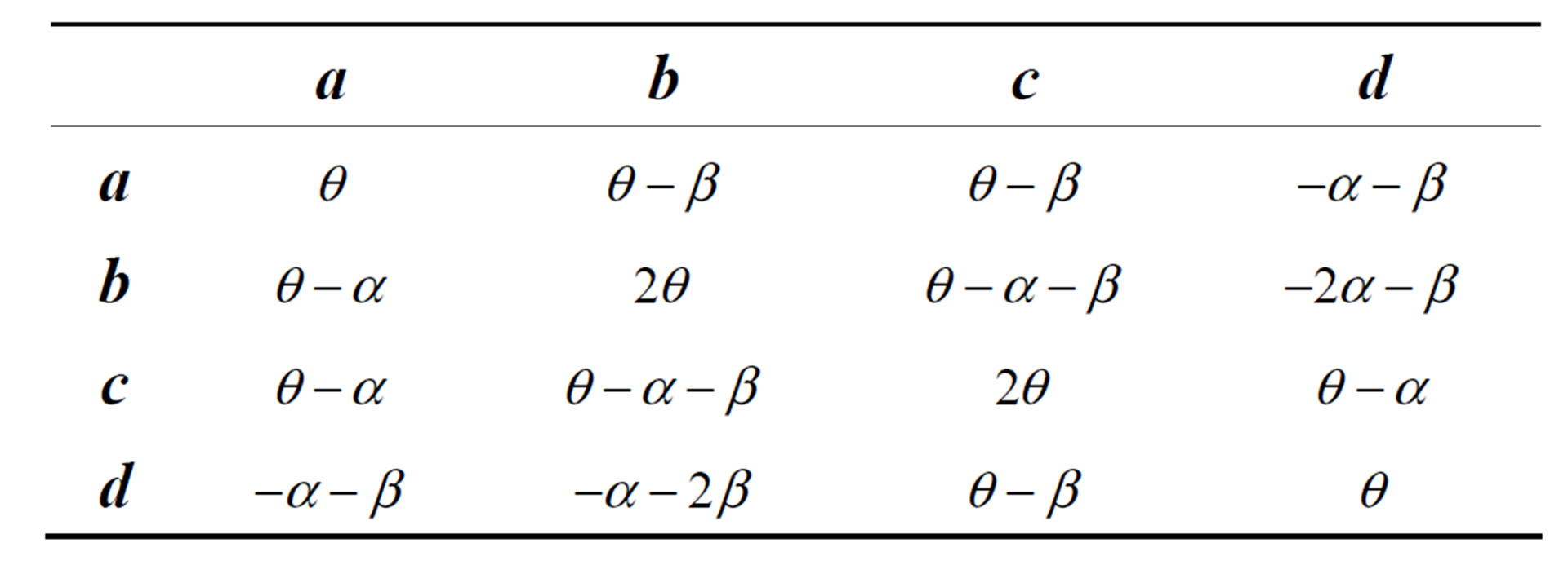
mentioned above could not be validated whatever the three constants (i.e.,  ,
, ![]() and
and ) would be when the FC model is used to measure the similarity. One might argue that this does not originate from the weakness of FC, but from the multiple meanings of the semantic features. The category COAST is related to two heterogeneous geo-objects, i.e., water in a sea and land near the sea.
Therefore, when images b or c are judged to be the most similar, one actually replace semantic feature island and building-area with a more general feature land. As mentioned above, Tversky ruled out this kind of multiple meanings of semantic features from his set-theoretic similarity by assuming that available features are independent and at a same level of generality. In image retrieval, the assumption is often hard to satisfy, in particular for the case that limited semantic features still need to be derived from low-level features or through interacting with users.
It can be concluded from the discussion mentioned-above that there exist two major limitations in the FC model: 1) the constants in the FC model can not adapt with the feature sets in comparison, but only regulate the relative salience between common and distinct features in a constant way; 2) semantics of features are assumed to be at a same level of generality in the FC model.
3. Self-Adaptive Feature Contrast Model
In this section, an adaptive feature contrast (AdaFC) model is presented to deal with the two limitations of the FC model, which have been drawn at the end of Section 2.
3.1. The Proposed Model
As shown in Equation (4), there exist two kinds of salience in the FC model: 1) the salience of individual feature; 2) the relative salience between common and distinct features. Therefore, a possible way to cope with the limitation of the FC model to directly model salience between features as suitable weights. [17] explored the former in the fuzzy feature contrast model. Although the three nonnegative constants in Equation (4) can reflect the relative salience between common and distinct features in a constant way, the constants are independent of any specific feature subset under measurement. [29] proposed a modified model to reflect the salience of individual feature when it acts as common or distinct feature. Following Daniel and Lee’s principle, the extreme case is that a feature is either purely common feature or a purely distinct feature. In other words, if a feature has been modeled as a purely distinct feature, it would not increase the similarity of the two objects even when it is a common feature in fact. Therefore, the weight defined by Daniel and Lee is independent of the fact that a feature is a common or distinct feature when comparing two objects.
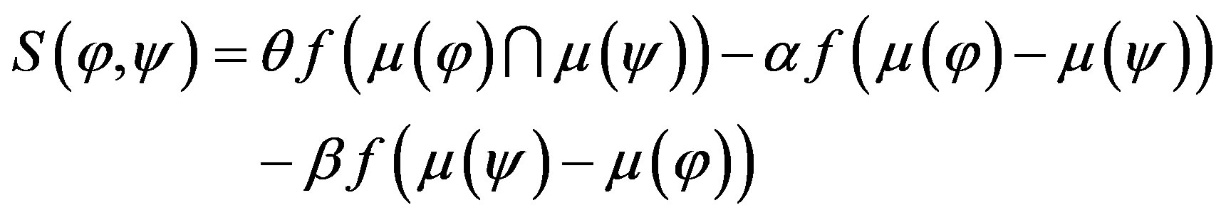
In this paper, we explore the relative salience between common and distinct features in the sense that the distinctiveness of distinct features is dependent on the two feature sets involved in current similarity assessment. Intuitionally speaking, some of distinct features would be distinguished if similarity measurement should be decreased significantly due to them. At the same time, we assume that common features are reliable and would always increase similarity measurements of images in a consistent way. Then, the relative salience between common and distinct features would be reduced to the salience of distinct features. To deal with the first limitation of the FC model, an adaptive feature contrast (AdaFC) model is given by
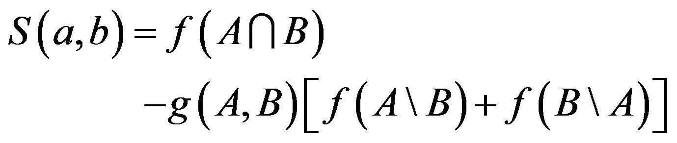 (10)
(10)
where  is an adaptive function describing the variation of relative salience of distinct features in similarity measurements.
Similar to both FC and FFC, the AdaFC also use both common and distinction to measure the similarity between two objects. Different from both FC and FFC, the AdaFC employs an adaptive function instead of the three constants as shown in both Equations (4) and (7) to balance the common and distinction between objects under consideration. Since the adaptive function g(A, B) in the AdaFC could change with the feature sets A and B, the first limitations mentioned at the last section would be eliminated. Please note that, instead of discrete feature sets in both the FC and AdaFC, fuzzy feature sets are used in the FFC. Consequently, it is unnecessary for the FFC to discretize continue visual feature vectors of images to a set of discrete feature set. In the AdaFC, we used an unsupervised clustering algorithm (i.e., Kmeans) to derive a set of feature set for each image.
3.2. The Adaptive Function
To deal with the second limitation, a two-layer clustering schema is employed to explore the various generality of features, so that the adaptive function 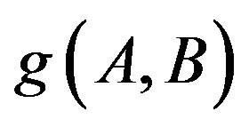 can be defined as a function of the two feature sets under measurement. As shown in Figure 3, the two-layer clustering schema consists of two clustering algorithm, i.e., KMEANS and Latent Dirichlet Allocation (LDA). The LDA [30] is a generative probabilistic hierarchical clustering model, which is originally developed to model collections of text documents. In this model, documents are represented as a finite mixture over latent topics, also called hidden aspects [31]. Each topic in turn is characterized by a distribution over words. The LDA has been extended to model image databases for image annotation [5], image categorization [6], and image retrieval [32,33]. When the LDA is used to model image databases, the terms documents and topics correspond to images and semantic objects, respectively. As a result, an image is represented as a mixture of topics, in other words, a
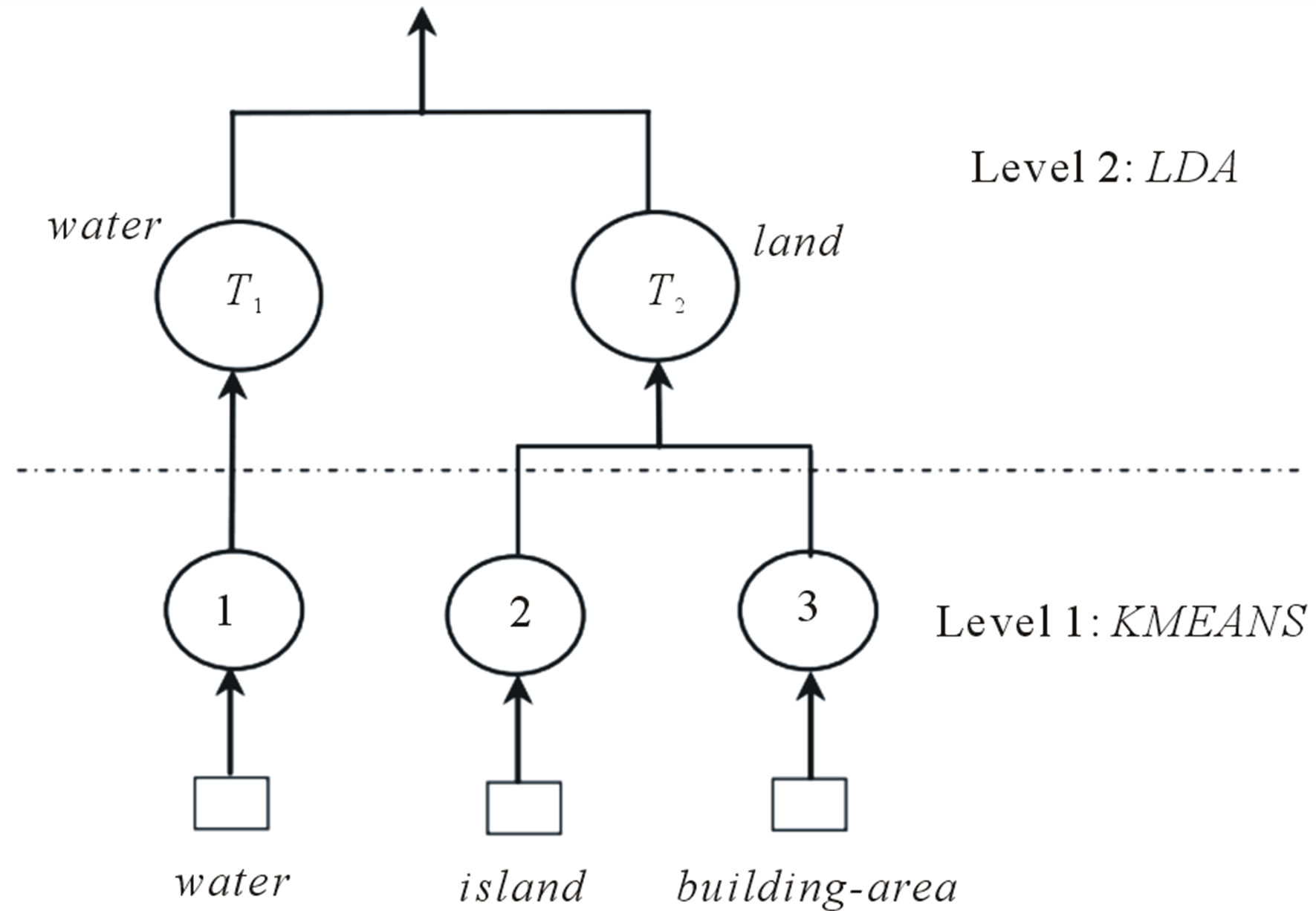
Figure 3. An illustration of two-layer hierarchical clustering process.
mixture of multiple semantic objects.
As shown in Figure 3, a two-layer clustering schema is used to illustrate a perfect hierarchical clustering process using a subset of images shown in Figure 2. At layer #1, a set of sub-images partitioning from large images are clustered using KMEANS algorithm, and each of them is allocated a label, e.g., 1, 2 and 3 in Figure 3. At layer #2, the LDA is used to learn semantic topics, e.g., T1 and T2 in Figure 3, and all images are represented as mixtures of the topics, e.g., MT. Each topic is a probabilistic distribution over the labels from KMEANS. For the sake of illustration, the topics T1 and T2 are tied a semantic name water and land, respectively. Note that we do not claim that the two-layer clustering in our experiments would exactly behave like that. In terms of visual consistence, the similarity judgment for sub-images within cluster 2 or 3 is more reliable than that within topic T2. In contrast, it is not the case for the dissimilarity judgment for sub-images among different clusters or topics. For instance, the dissimilarity judgment of sub-images between Topic T1 and T2 is more reliable than that between clusters 2 and 3. The reason is that clusters 2 and 3 share a same semantic, i.e., both of them belong to a more general concept land. In the proposed method, cluster labels instead of topic labels are used as features to represent images, because their similarity judgments are more reliable, and cluster labels would be at a same level of salience from the viewpoint of similarity measurement. At the same time, the adaptive function  based on topic mixtures is proposed to regulate the role of dissimilarity judgments in any two images a and b
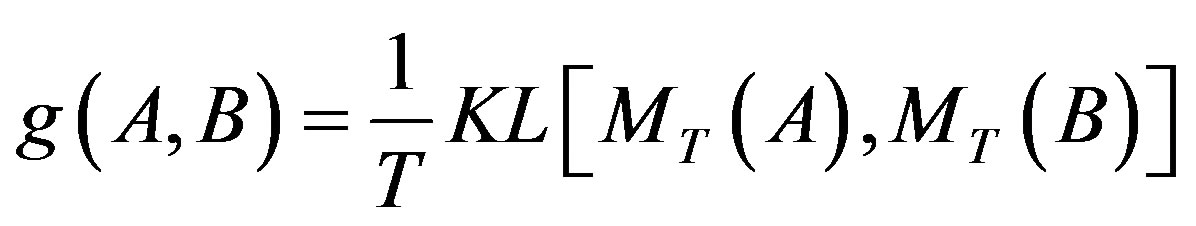 (11)
(11)
where A and B are the sets of cluster labels of image a and b, respectively; 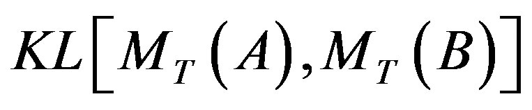 is the Kullback-Leibler divergence of topic mixture coefficients
 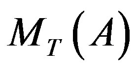 and
and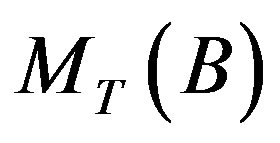 ; T is the number of topics.
According to the definition given in Equation (11), adaptive function 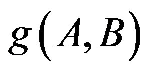 can be used to solve the multiple meanings of features by regulating the role of distinct features. For the four images shown in Figure 2, the expected behavior of the AdaFC model is as follows: 1) when the similarity between images b and c is measured, it will be a smaller value, so that the distinction of distinct features is trivial and should be totally ignored or tolerated; 2) when measuring the similarity of images a and b (or c and d), it will be a larger value, so that distinct features would be distinguished by allocating a larger weight.
4. Experiments and Discussion
The goal of content-based image retrieval is to obtain images with content similar to a given sample image. In this section, the AdaFC model is evaluated in the framework of content-based image retrieval for satellite images database. All experiments are performed on a database consisting of over 10,000 SPOT5 PAN images with size of 512 × 512. The database is made of five scenes (i.e., CITY, COAST, FIELD, MOUNTAIN, SEA). Except the scene COAST, only one typical semantic object occurs in the image. For instance, building-area (resp., field, mountain, water) occurs in the scene CITY (resp., FIELD, MOUNTAIN, SEA). Among all scenes in the image database, COAST might be the most difficult to well retrieve using similarity measurements. The difficulty originates from two aspects: 1) images include two different semantics, i.e., water and land; 2) the semantic land might occur in different forms, e.g., island or building-area.
4.1. Image Representation and Similarity Measures
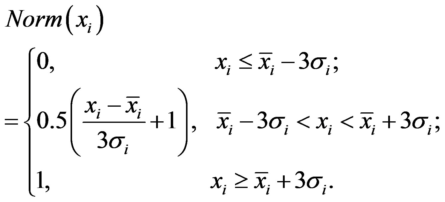
As shown in Figure 1, image representation can be divided into 4 steps: partition, feature extraction, clustering and representation. Each image is partitioned into 64 sub-images with size of 64 × 64. Then, a low-level feature is extracted from each sub-image. The low-level features include Gabor texture, gray histogram and gradient histogram. Texture feature is the average and variance of Gabor filters (2 scales and 5 directions) [34,35]. Therefore, each region corresponds to a 20-dimensional texture feature vector. In addition, after a gray histogram of 256 bins has been extracted from each region, the principal component analysis is employed to reduce the dimension of histogram to 20 dimensions by keeping more than 95% energy. The gradient histogram is created by first computing the gradient magnitude and orientation at each pixel in a sub-image. Then, gradient magnitudes of all pixels are accumulated into the orientation histogram, in which there are 18 orientations equally partitioning a circle. In total, each sub-image corresponds to a 58-dimensional low-level feature vector. The three types of low-level features are individually normalized using
 (12)
(12)
where ,
,  and
and  are ith dimensional feature value, mean and variance.
Based on the extracted low-level features, the twolayer clustering algorithm as shown in Figure 3 is used to allocate a label for each subimage. Using all labels of sub-images in the image, images are represented as label vectors or sets. Apart from the extended model, two kinds of similarity measures are selected as benchmark methods in our experiments. One is the FC model, and the other is COV coupled with Kullback-Leibler divergence. Specifically, four kinds of similarity measures in our experiments are described as follows:
1) AdaFC: the extended model is defined in Equation (10), where the feature set for each image is a set of cluster label allocated by KMEANS, i.e., layer #1 clustering in Figure 3, and the adaptive function defined in Equation (11) is dependent on the clustering from LDA, i.e., layer #2 clustering in Figure 3;
2) FC: The feature contrast model is given in Equation (4), where the feature set for each image is a set of cluster label allocated by KMEANS, i.e., layer #1 clustering in Figure 3;
3) FFC: The fuzzy feature contrast model is given in Equation (7), where the feature vector for each image is the 58-dimensional low-level feature.
4) KL: It is the Concept Occurrence Vector coupled with Kullback–Leibler divergence, where the vector is the topic mixture due to layer #2 clustering in Figure 3. It is a state-of-the-art approach for image retrieval using probabilistic topic models [14,32].
4.2. Experimental Results and Discussion
Retrieval Precision (RP) and recall are used to evaluate the effectiveness of similarity measures. Given M retrieved images, assume there exist P positive images in the M images, and TP positive images in the image database. The RP is the ratio of number of positive images to that of retrieved images, i.e., P/M. The recall is the ratio of number of positive and retrieved images to that of all positive images in the image database, i.e., P/TP. In addition, a Receiver Operating Characteristic (ROC) and its Area Under Curve (AUC) are also employed to evaluate the performance of the similarity measures. In the ROC, the false positive rate is the ratio of the number of N negative images in the M retrieved images to that of TN negative images in the image database, i.e., N/TN. The hit rate (i.e., true positive rate) is equal to the recall.
In our experiments, the retrieval performance might be influenced by some parameters, such as the number of topics in the LDA, number of clusters in the KMEANS, the constants defined in the FC model. In the following, we discuss these parameters using experimental results.
4.2.1. The Number of Topics in the LDA
The perplexity is frequently used to assess the performance of LDA in the context of both text and image modeling [14,30,31]. It measures the performance of the model on a held out dataset ![]() and is defined by
and is defined by
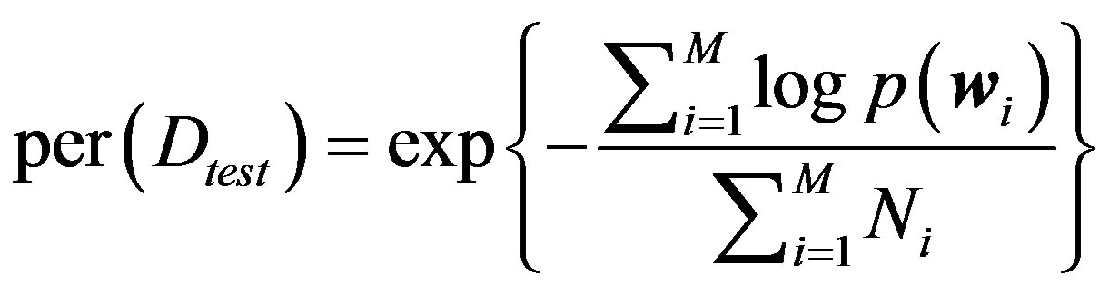 (13)
(13)
where  and
and  are the set of “words” (i.e., cluster labels from KMEANS) and the number of words in ith image;
  is the likelihood of ith image under the estimated model.
A five-fold cross-validation is employed to determine the number of topics. Specifically, we use 20% images in the image database to train LDA models over different numbers of topics, and respectively calculate the perplexity on the 80% holdout images using Equation (13). The averaged value and standard variance of perplexities over the five-fold subsets is shown in Figure 4. It can be seen from Figure 4 that the perplexity decreases with an increasing number of topics. Specifically, when the number of topics is less then 15, the perplexity rapidly decreases. This indicates that the model does not fit the holdout data every well. However, when the number of topics is larger than 15, the perplexity becomes relatively stable. In other words, the fitness can not be furthermore improved when the number of topics is larger than 15. Therefore, the number of topics is set to 15 in our experiments.
4.2.2. The Number of Clusters in the KMEANS
Because cluster labels are employed to represent images, the number of clusters is an important parameter for the “quality” of representation. Although some principles could be employed to select a suitable number of clusters, e.g., Minimum Description Length, what we are interested in is not to choose an optimal number, but expect that the extended model would consistently improve the effectiveness of FC model independent of the number of clusters to some extent.
The retrieval precisions and recall, shown in the four plots of Figures 5 and 6 respectively, are calculated when the number of clusters is equal to 100, 500, 1000 and 1500, respectively. Although the performances of similarity measures do change with the number of clusters, the relative performances among different categories do not change for a given similarity measure. For example, the retrieval precision of COAST is always the lowest one among the five categories. The retrieval precisions of both MOUNTAIN and SEA are always higher than 90%.
For the category COAST, the retrieval precision of the AdaFC is near to 80%, and the AdaFC outperforms FC up to over 10% retrieval precision. For other categories, the performance of AdaFC is larger than or almost equal to that of both FC and FFC. In other words, the proposed adaptive function given in Equation (11) could consistently improve the performance of FC. As we known, the
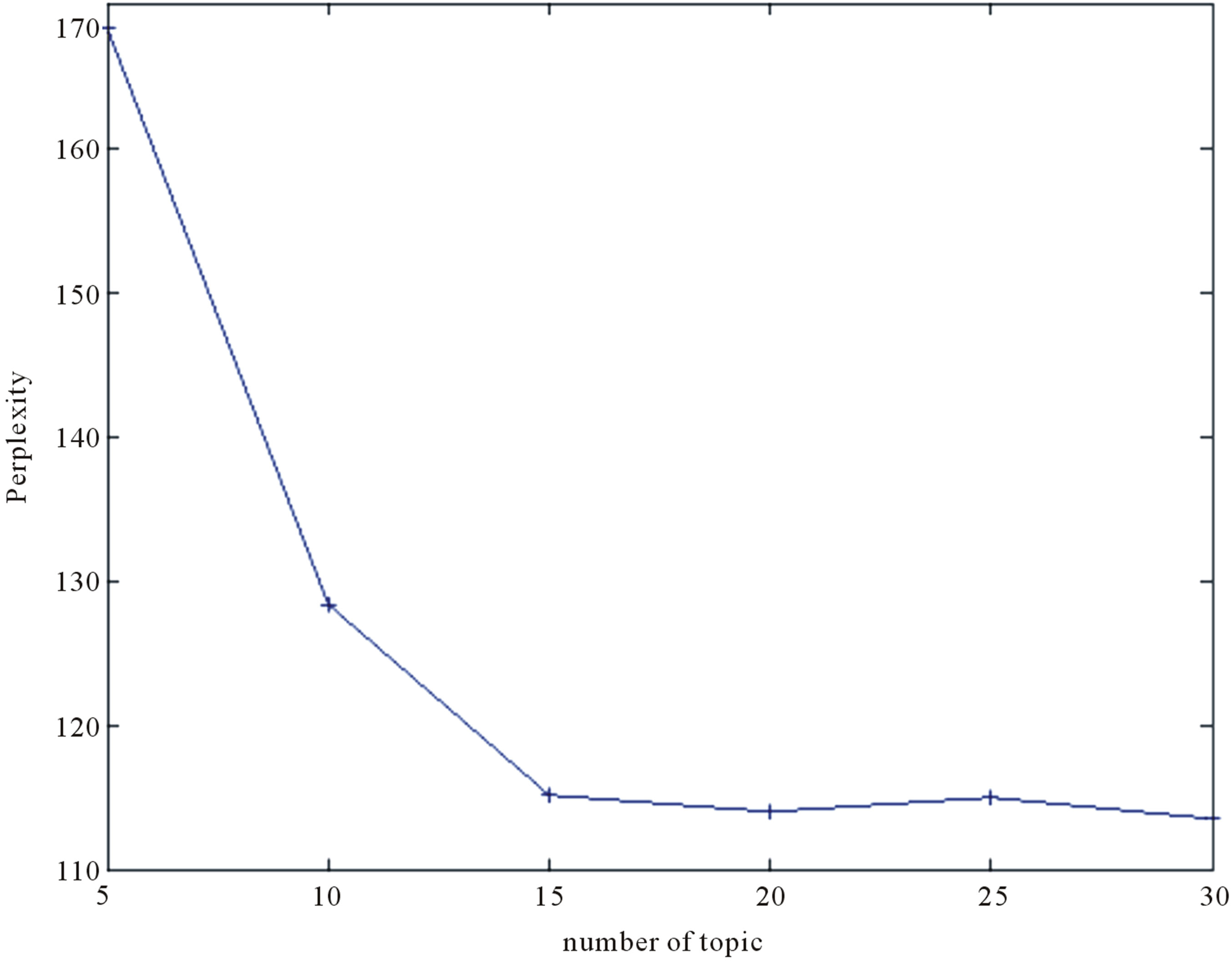
Figure 4. Perplexity vs. number of topic.
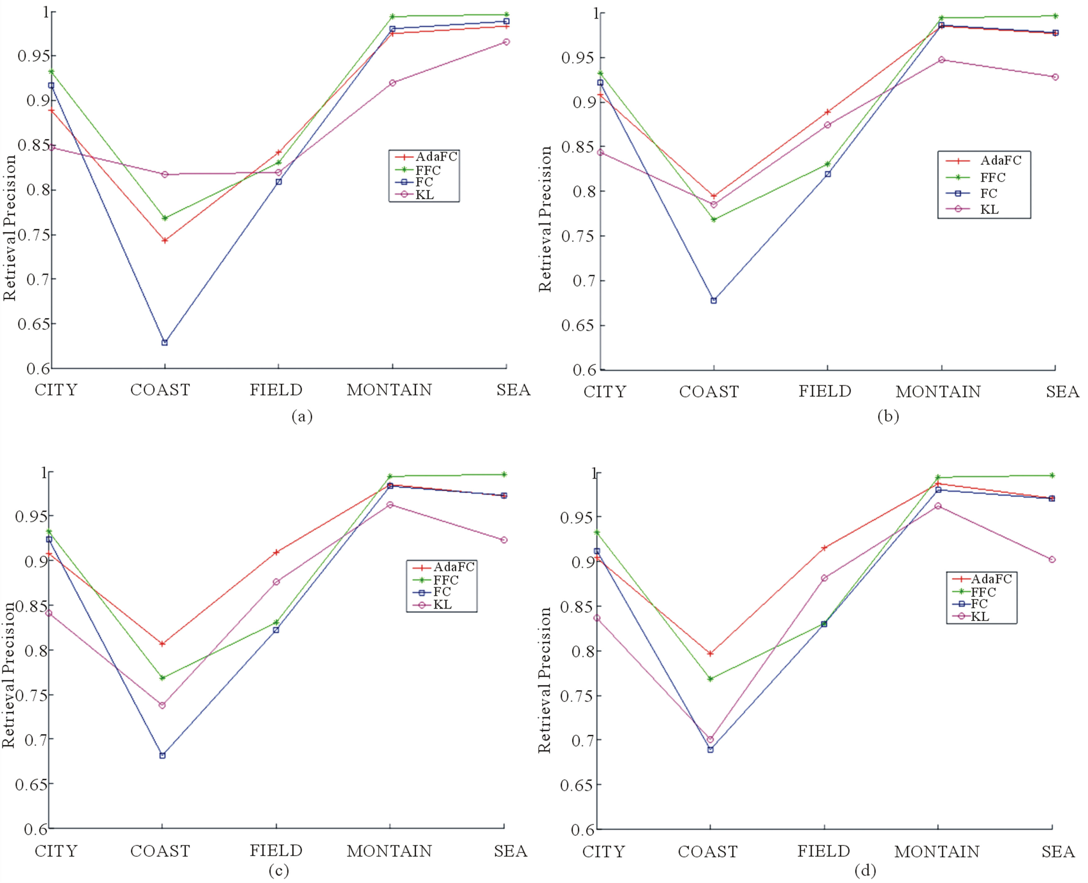
Figure 5. Retrieval precision using AdaFC, FFC, FC and KL. (a) Number of clusters = 100; (b) Number of clusters = 500; (c) Number of clusters = 1000; (d) Number of clusters = 1500.
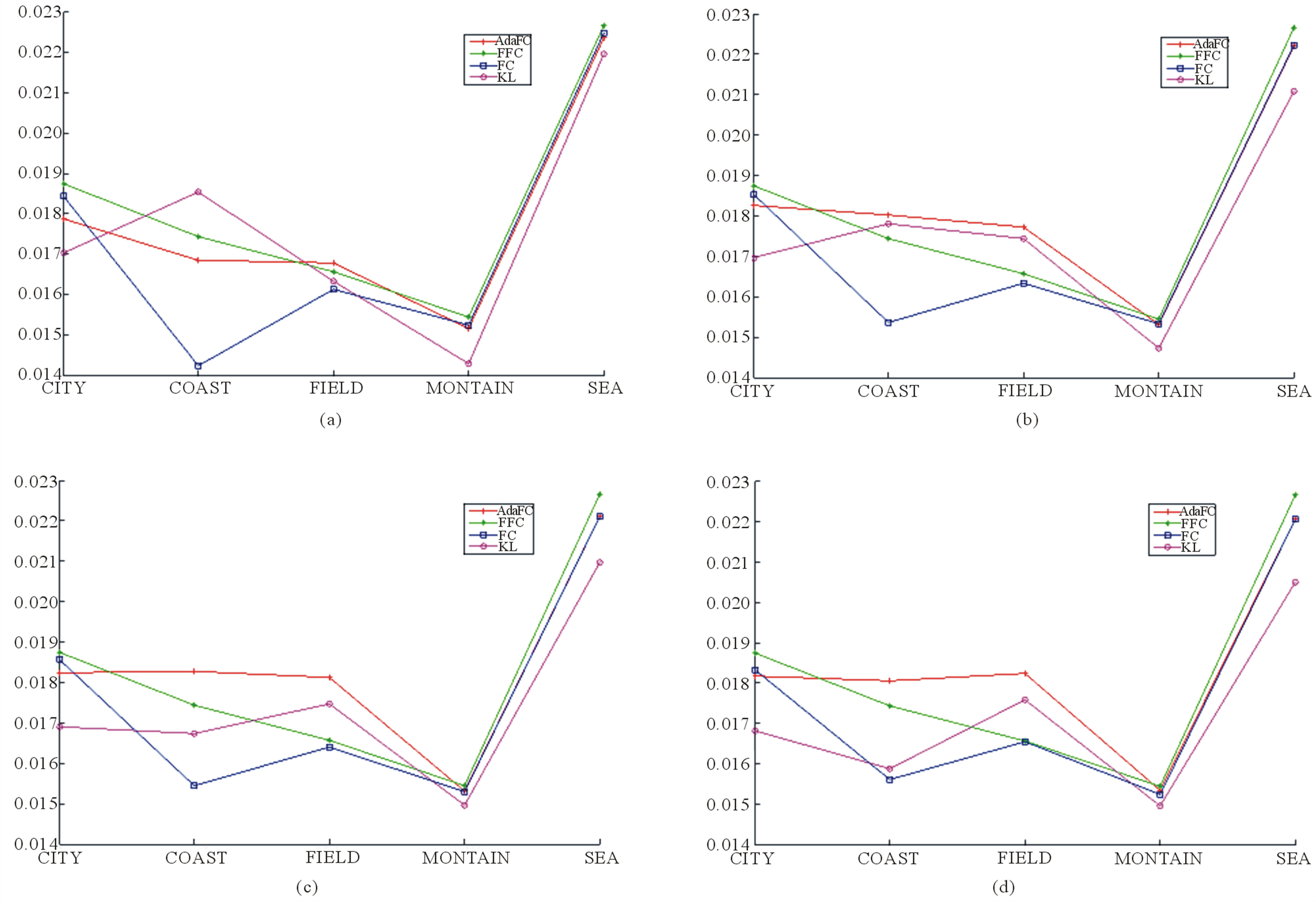
Figure 6. Retrieval recall using AdaFC, FFC, FC and KL. (a) Number of clusters = 100; (b) Number of clusters = 500; (c) Number of clusters = 1000; (d) Number of clusters = 1500.
adaptive function is a function of Kullback–Leibler divergence between the topic mixture coefficients for the two images. As shown in Figure 5, there is another similarity measure, i.e., Kullback-Leibler divergence between the topic mixture coefficients, which has been widely applied to image or text retrieval [14,32]. Like the AdaFC, the retrieval precision based on the KL is larger than that based on the FC for the categories COAST and FIELD. However, unlike the AdaFC, the performance of KL is significantly worse than that of FC for the rest of categories, i.e., CITY, MOUNTAIN and SEA. Therefore, it can be concluded from these results that the AdaFC inherits the merits from both the FC and the KL. In other words, it is the two-layer clustering schema (KMEANS + LDA) that makes the adaptive become a successful practice.
Figure 7 lists the Receiver Operating Characteristic and its Area Under Curve (AUC). In terms of the AUC, the AdaFC outperforms both the FC and KL whatever the number of cluster is. The AdaFC is still comparable to the FFC when the number of cluster is equal to 1500. In addition, when the false positive rate is less than 0.2, the true positive of the AdaFC is always higher than that of the FFC.
4.2.3. Constant Parameters vs. Adaptive Function
The three constants in Equation (4), i.e.,  ,
, ![]() and
and  do reflect the relative salience of common features (i.e.,
 ) and two kinds of distinct feature (i.e.,
  and
and ). One might argue that the FC could perform as well as the AdaFC after the constants are carefully selected. In the following, two experiments are made to refute this argument.
It can be seen from comparing Equation (10) and Equation (4) that there exist two assumptions about the relative salience in similarity measurements, i.e.,  ,
,  and the constant
 ![]() is replaced with an adaptive function
is replaced with an adaptive function  in Equation (10). To fairly compare the performance between the FC and AdaFC, we assume that
 ,
,  and the constant
 ![]() increase from 0 to 1 at the step of 0.1 in the first experiment. Table 2 lists the retrieval precisions for the FC when
increase from 0 to 1 at the step of 0.1 in the first experiment. Table 2 lists the retrieval precisions for the FC when  and the
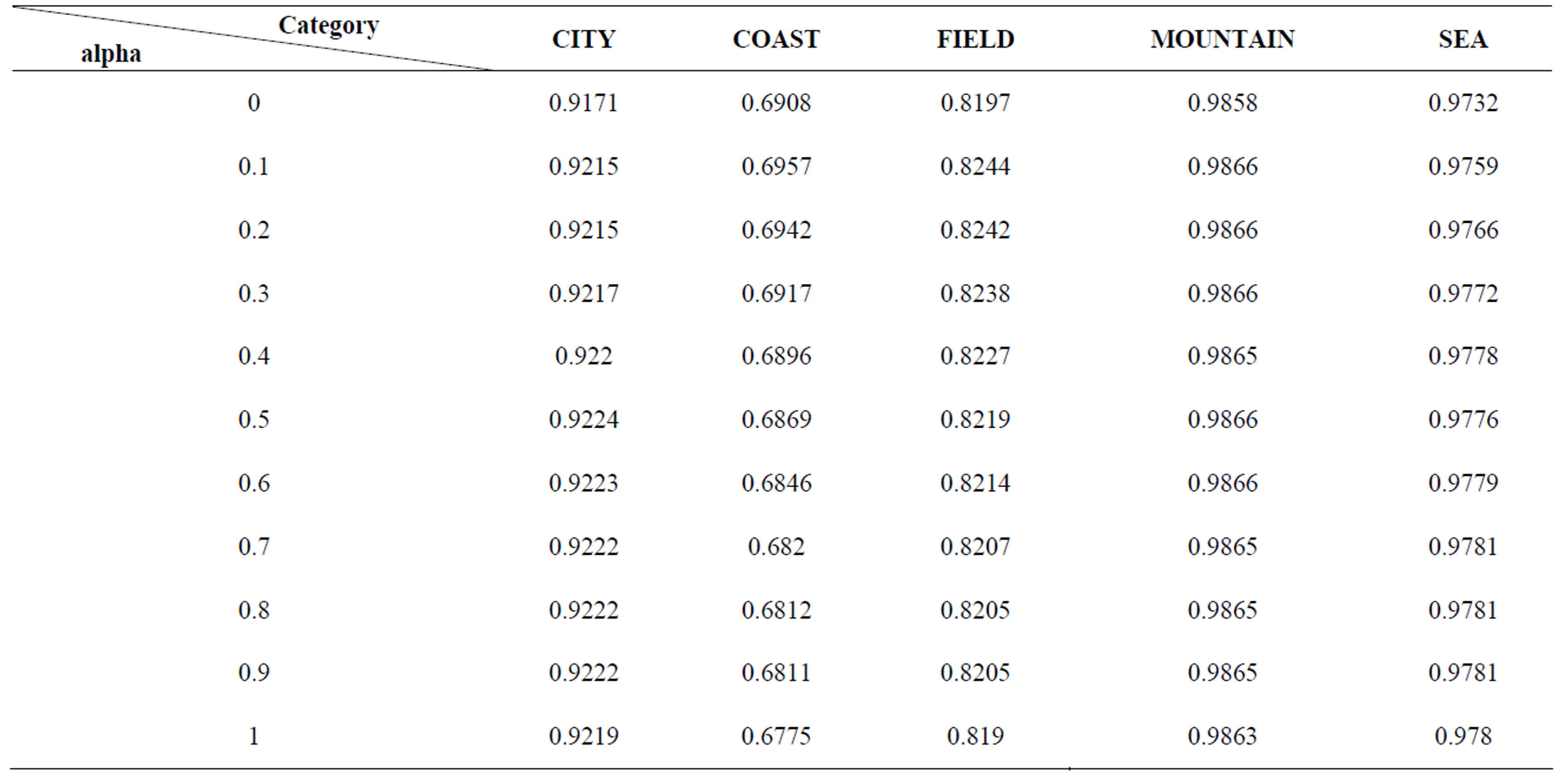
 ![]() increase from 0 to 1. It can be seen from Table 2 that: (1) the retrieval precision does not change very much for all of six categories when the
increase from 0 to 1. It can be seen from Table 2 that: (1) the retrieval precision does not change very much for all of six categories when the ![]() increase from 0 to 1; (2) for the category COAST, the highest retrieval precision is still lower than 70%. However, as shown in Figure 5, the retrieval precision of AdaFC is near to 80%. Therefore, we an not expect that the performance of the AdaFC can
increase from 0 to 1; (2) for the category COAST, the highest retrieval precision is still lower than 70%. However, as shown in Figure 5, the retrieval precision of AdaFC is near to 80%. Therefore, we an not expect that the performance of the AdaFC can
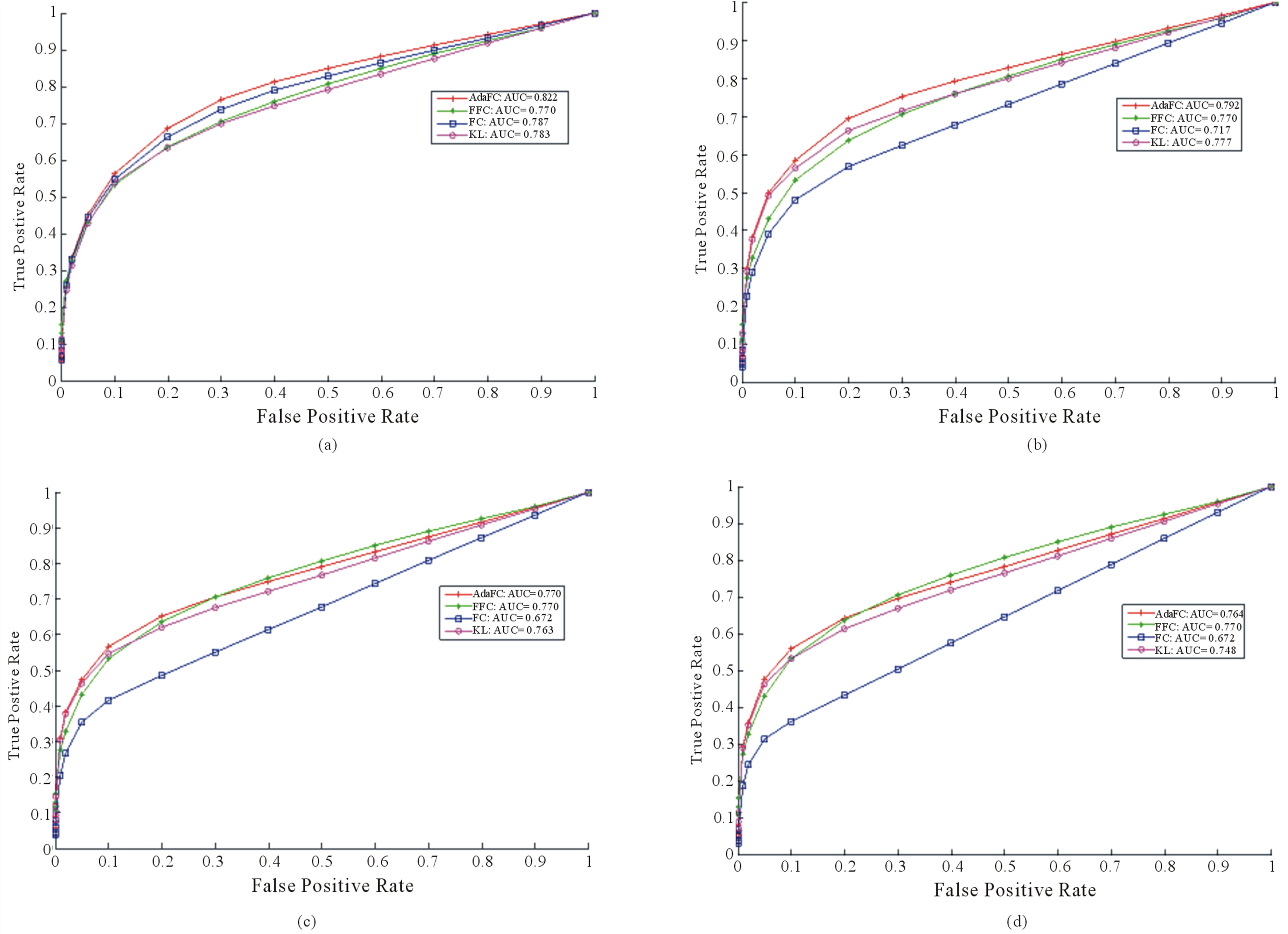
Figure 7. The ROC of the AdaFC, FFC, FC and KL. (a) Number of clusters = 100; (b) Number of clusters = 500; (c) Number of clusters = 1000; (d) Number of clusters = 1500.
Table 2. Retrieval precisions using the FC when theta =1 and alpha varies from 0 to 1.
be obtained by the FC through selecting a suitable value for the![]() , since the adaptive function
, since the adaptive function  in the AdaFC is not a constant, but is adaptive with both A and B.
The other question is whether we could obtain the same performance of the AdaFC through changing the two kinds of constants, i.e.,  for common features and
![]() ,
, for distinctive features, at the same time. To answer this question, a second experiment is made to evaluate the effect when the constant
  for comment features and
 ![]() (or
(or ) for distinct features are a convex combination, i.e.,
  and
and . Table 3 list the retrieval precisions for the FC when the
  increases from 0 to 1,
  and
and . For the category COAST, the highest retrieval precision is still lower than 70%. Although only a simple linear convex combination is tested in this experiment, we still could believe that the performance of the AdaFC can not be obtained using the FC only by selecting a suitable set of constants.
4.2.4. Retrieval Results
Apart from the statistical retrieval performance mentioned above, two intuitional retrieval results are shown in Figures 8(a) and (b), where we used a same querying image (i.e., the top-left COAST image in Figure 8(a) or Figure 8(b)) coupled with two similarity measures (i.e., AdaFC and FC). As shown Figure 8(a), all of the top 40 most similarity images belong to the same category as the querying image, i.e., COAST. In contrast, as shown in Figure 8(b), both one CITY image and two SEA images are incorrectly retrieved the FC as a similarity measurement. Since there are two geo-objects in the querying image, i.e., water and building-area, both CITY and COAST images could be retrieved using the FC. The contrast between the two retrieval results intuitionally shows the improvement of AdaFC over FC.
5. Conclusion
In this paper, we extend Tversky’s FC model to the situation that semantic features might not be at a same level of generality. Unlike common features, the role of distinct features might be switched from one state to another in the situation. Therefore, an adaptive function is employed to simulate the switch of distinct features in satellite image retrieval. Experimental results show that the retrieval precision can be improved more than 10% for satellite images with heterogeneous objects, e.g., COAST images. However, the solution is still far from achieving fluent feature selection of human, which actually is a process of feature selection for a given task. Therefore, the key is to discover the relevance of features to the goal when comparing two objects. However, the term feature selection (i.e., select relevant features for objects to be compared) is different from that used in machine learning (i.e., select a subset of features for all objects from a feature set). It seems to be a “local” or real-time feature selection in the sense that selected features would not be used in a consistent way. Therefore, the feature switch of human is too ideal to realize in real applications. Any way, we attempt to approach it in some limited situations. The next step is to explore the relevance of features during feature extraction. Then, features could be utilized in a more local or real-time way.
Table 3. Retrieval precisions using the FC when theta = 1-alpha and theta varies from 0 to 1.
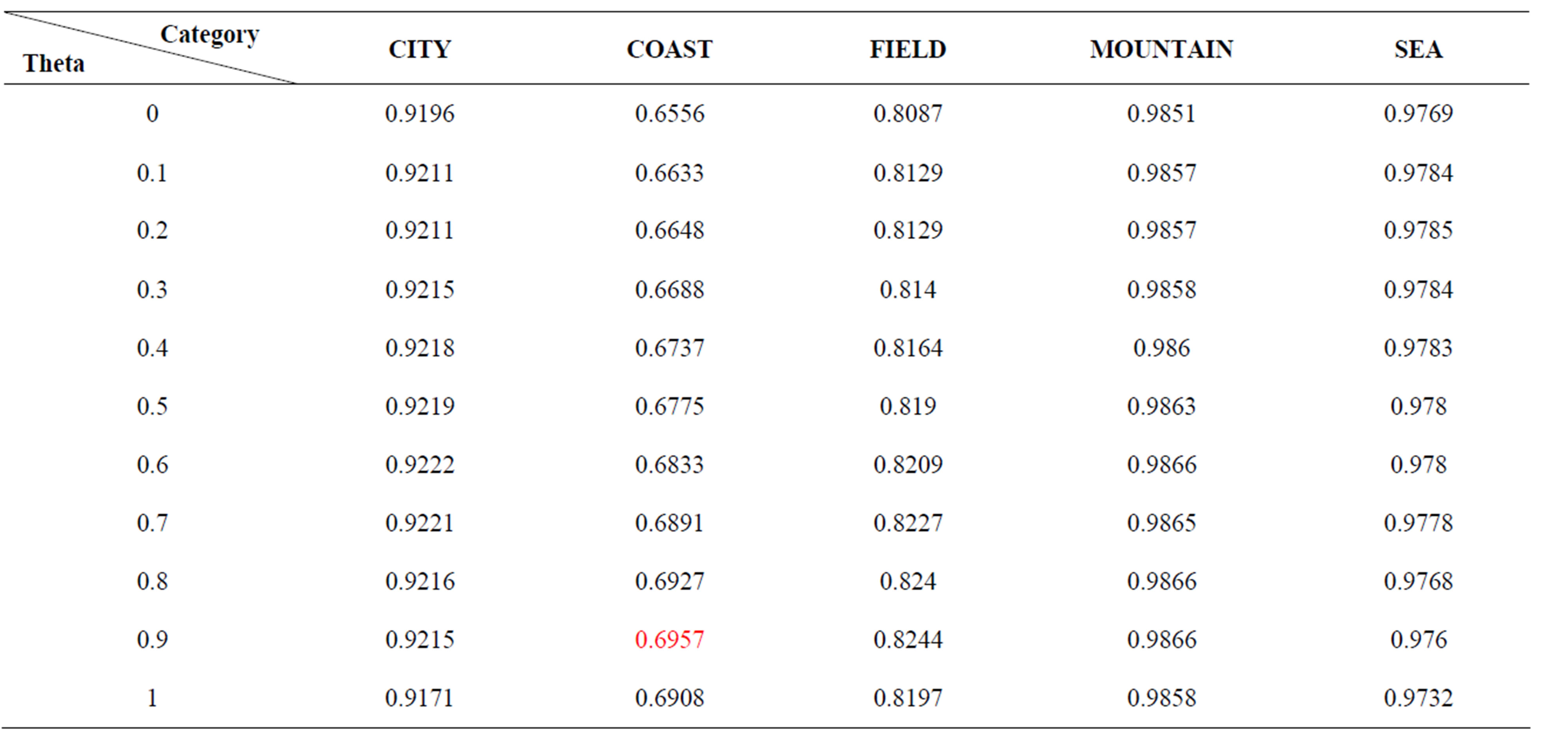
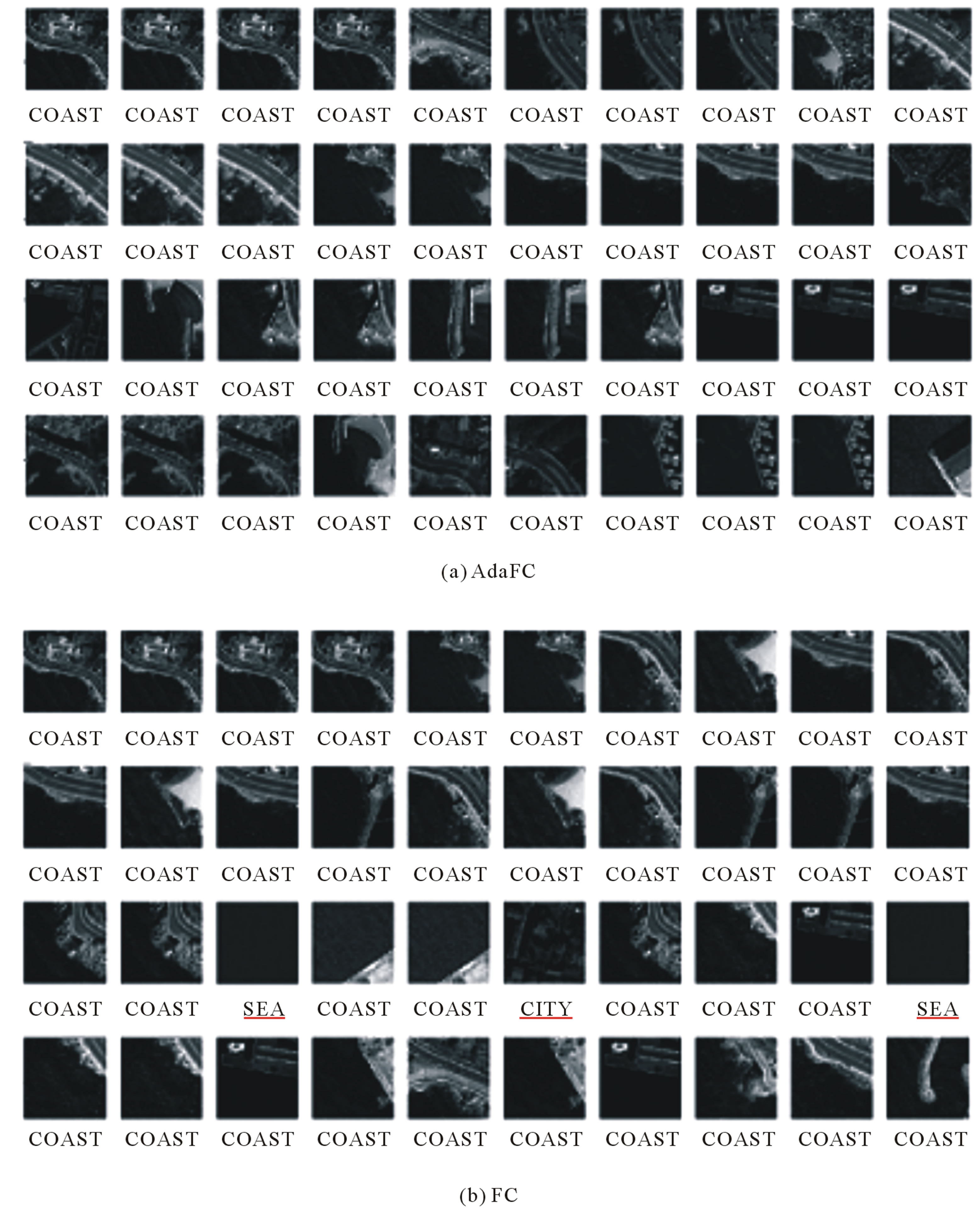
Figure 8. (a) Retrieval results using AdaFC where all of retrieved images are COAST images; (b) Retrieval results using FC where there are two SEA images and CITY image are incorrectly retrieved.
6. Acknowledgements
This work is in part supported by National Natural Science of China (No. 40901217), Program for New Century Excellent Talents in University (No. NECT-11-0039) and National High Technology Research and Development Program of China (No. 2012AA121302).
REFERENCES
- M. Datcu, K. Seidel and M. Walessa, “Spatial Information Retrieval from Remote-Sensing Images. I. Information Theoretical Perspective,” IEEE Transactions on Geoscience and Remote Sensing, Vol. 36, No. 5, 1998, pp. 1431-1445. doi:10.1109/36.718847
- M. Datcu, H. Daschiel, A. Pelizzari, M. Quartulli, A. Galoppo, A. Colapicchioni, M. Pastori, K. Seidel, P. G. Marchetti and S. D’Elia, “Information Mining in Remote Sensing Image Archives: System Concepts,” IEEE Transactions on Geoscience and Remote Sensing, Vol. 41, No. 12, 2003, pp. 2923-2936. doi:10.1109/TGRS.2003.817197
- B. S. Manjunath, J. R. Ohm, V. V. Vasudevan and A. Yamada, “Color and Texture Descriptors,” IEEE Transactions On Circuits and Systems for Video Technology, Vol. 11, No. 6, 2001, pp. 703-715. doi:10.1109/76.927424
- J. Li and J. Wang, “IRM: Integrated Region Matching for Image Retrieval,” Proceedings ACM Multimedia, Los Angeles, 30 October-3 November 2000, pp. 147-156.
- K. Barnard, P. Duygulu and D. Forsyth, “Matching Words and Pictures,” Journal of Machine Learning Research, Vol. 3, No. 2, 2007, pp. 1107-1135.
- G. Carneiro, A. B. Chan, P. J. Moreno and N. Vasconcelos, “Supervised Learning of Semantic Classes for Image Annotation and Retrieval,” IEEE Transactions on Pattern Analysis and Machine Intelligence, Vol. 29, No. 3, 2007, pp. 394-410. doi:10.1109/TPAMI.2007.61
- A. Mojsilovic, J. Gomes and B. Rogowitz, “SemanticFriendly Indexing and Quering of Images Based on the Extraction of the Objective Semantic Cues,” International Journal of Computer Vision, Vol. 56, No. 1-2, 2004, pp. 79-107. doi:10.1023/B:VISI.0000004833.39906.33
- J. Vogel and B. Schiele, “Semantic Modeling of Natural Scenes for Content-Based Image Retrieval,” International Journal of Computer Vision, Vol. 72, No. 2, 2007, pp. 133-157. doi:10.1007/s11263-006-8614-1
- J. Z. Wang, J. Li and G. Wiederhold, “SIMPLIcity: Semantics-Sensitive Integrated Matching for Picture Libraries,” IEEE Transactions on Pattern Analysis and Machine Intelligence, Vol. 23, No. 9, 2001, pp. 947-963. doi:10.1109/34.955109
- M. Ferecatu, N. Boujemaa and M. Crucianu, “Semantic Interactive Image Retrieval Combining Visual and Conceptual Content Description,” Multimedia Systems, Vol. 13, No. 5-6, 2008, pp. 309-322. doi:10.1007/s00530-007-0094-9
- X. F. He, O. King and W. Y. Ma, “Learning a Semantic Space from User’s Relevance Feedback for Image Retrieval,” IEEE Transactions on Circuits and Systems for Video Technology, Vol. 13, No. 1, 2003, pp. 39-48. doi:10.1109/TCSVT.2002.808087
- S. Santini, A. Gupta and R. Jain, “Emergent Semantics through Interaction in Image Databases,” IEEE Transactions on Knowledge and Data Engineering, Vol. 13, No. 3, 2001, pp. 337-351. doi:10.1109/69.929893
- C. Zhang and T. S. Chen, “An Active Learning Framework for Content-Based Information Retrieval,” IEEE Transactions on Multimedia, Vol. 4, No. 2, 2002, pp. 260-268. doi:10.1109/TMM.2002.1017738
- E. Hörster, “Topic Models for Image Retrieval on LargeScale Databases,” Dissertation, University of Augsburg, 2009.
- A. Tversky, “Features of Similarity,” Psychological Review, Vol. 84, No. 4, 1977, pp. 327-352. doi:10.1037/0033-295X.84.4.327
- S. Santini and R. Jain, “Similarity Measures,” IEEE Transactions on Pattern Analysis and Machine Intelligence, Vol. 21, No. 9, 1999, pp. 871-883. doi:10.1109/34.790428
- H. Tang, T. Fang, P. J. Du and P. F. Shi, “Intra-Dimensional Feature Diagnosticity in the Fuzzy Feature Contrast Model,” Image and Vision Computing, Vol. 26, No. 6, 2008, pp. 751-760. doi:10.1016/j.imavis.2007.08.009
- Y. Chen and J. Z. Wang, “A Region-Based Fuzzy Feature Matching Approach to Content-Based Image Retrieval,” IEEE Transactions on Pattern Analysis and Machine Intelligence, Vol. 24, No. 9, 2002, pp. 1252-1267. doi:10.1109/TPAMI.2002.1033216
- Y. Chen and J. Z. Wang, “Image Categorization by Learning and Reasoning with Regions,” Journal of Machine Learning Research, Vol. 5, 2004, pp. 913-939.
- S. Lazebnik, C. Schmid and J. Ponce, “Beyond Bags of Features: Spatial Pyramid Matching for Recognizing Natural Scene Categories,” IEEE Computer Society Conference on Computer Vision and Pattern Recognition, Vol. 2, 2006, pp. 2169-2178.
- F. F. Li and P. Pietro, “A Bayesian Hierarchical Model for Learning Natural Scene Categories,” IEEE Computer Society Conference on Computer Vision and Pattern Recognition, Vol. 2, 2005, pp. 524-531.
- P. Quelhas, F. Monay and J. M. Odobez, “Modeling Scenes with Local Descriptors and Latent Aspects,” IEEE International Conference on Computer Vision, Vol. 1, 2005, pp. 883-890.
- A. Bosch, X. Munoz and R. Marti, “Which Is the Best Way to Organize/Classify Image by Content,” Image and Vision Computing, Vol. 25, No. 3, 2007, pp. 778-791. doi:10.1016/j.imavis.2006.07.015
- G. Csurka, C. Dance, L. Fan, J. Williamowski and C. Bray, “Visual Categorization with Bags of Keypoints,” ECCV Workshop on Statistical Learning in Computer Vision, Prague, 2004.
- R. L. Goldstone, “Similarity,” In: R. Wilson and F. C. Keil, Eds., MIT Encyclopedia of the Cognitive Sciences, MIT Press, Cambridge, 1999, pp. 763-765.
- R. N. Shepard, “Toward a Universal Law of Generalization for Psychological Science,” Science, Vol. 237, No. 4820, 1987, pp. 1317-1323. doi:10.1126/science.3629243
- R. L. Goldstone, “Alignment-Based Nonmonotonicities in Similarity,” Journal of Experimental Psychology: Learning, Memory, and Cognition, Vol. 22, No. 4, 1996, pp. 988-1001. doi:10.1037/0278-7393.22.4.988
- U. Hahna, N. Chater and L. B. Richardson, “Similarity as Transformation,” Cognition, Vol. 87, No. 1, 2003, pp. 1-32. doi:10.1016/S0010-0277(02)00184-1
- J. N. Daniel and M. D. Lee, “Common and Distinctive Features in Stimulus Similarity: A Modified Version of the Contrast Model,” Psychologic Bulletin & Review, Vol. 11, No. 6, 2004, pp. 961-974. doi:10.3758/BF03196728
- D. M. Blei, A. Y. Ng and M. I. Jordan, “Latent Dirichlet Allocation,” Journal of Machine Learning Research, Vol. 3, No. 2, 2003, pp. 993-1022.
- T. Hofmann, “Unsupervised Learning by Probabilistic Latent Semantic Analysis,” Machine Learning, Vol. 42, No. 1-2, 2001, pp. 177-196.
- R. Lienhart and M. Slaney, “pLSA on Large Scale Image Databases,” IEEE International Conference on Acoustics, Speech and Signal Processing, Honolulu, 15-20 April 2007, pp. 1217-1220.
- E. Hörster, R. Lienhart and M. Slaney, “Image Retrieval on Large-Scale Image Databases,” ACM International Conference on Image and Video Retrieval (CIVR), Amsterdam, 2007, pp. 17-24.
- B. S. Manjunath and W. Y. Ma, “Texture Features for Browsing and Retrieval of Image Data.,” IEEE Transactions on Pattern Analysis and Machine Intelligence, Vol. 18, No. 8, 1996, pp. 837-842. doi:10.1109/34.531803
- Y. Deng and B. S. Manjunath, “Unsupervised Segmentation of Color-Texture Regions in Images and Video,” IEEE Transactions on Pattern Analysis and Machine Intelligence, Vol. 23, No. 8, 2001, pp. 800-810. doi:10.1109/34.946985
NOTES
*Corresponding author.