Advances in Remote Sensing
Vol.2 No.4(2013), Article ID:40777,13 pages DOI:10.4236/ars.2013.24036
A Comprehensive Evaluation of PAN-Sharpening Algorithms Coupled with Resampling Methods for Image Synthesis of Very High Resolution Remotely Sensed Satellite Data
Polar Remote Sensing Department, Earth System Sciences Organization (ESSO), National Centre for Antarctic and Ocean Research (NCAOR), Ministry of Earth Sciences, Government of India, Headland Sada, Gao, India
Email: shridhar.jawak@gmail.com; shridhar.jawak@ncaor.gov.in
Copyright © 2013 Shridhar D. Jawak, Alvarinho J. Luis. This is an open access article distributed under the Creative Commons Attribution License, which permits unrestricted use, distribution, and reproduction in any medium, provided the original work is properly cited.
Received August 1, 2013; revised September 1, 2013; accepted September 8, 2013
Keywords: PAN-sharpening; WorldView-2; resampling methods
ABSTRACT
The merging of a panchromatic (PAN) image with a multispectral satellite image (MSI) to increase the spatial resolution of the MSI, while simultaneously preserving its spectral information is classically referred as PAN-sharpening. We employed a recent dataset derived from very high resolution of WorldView-2 satellite (PAN and MSI) for two test sites (one over an urban area and the other over Antarctica), to comprehensively evaluate the performance of six existing PAN-sharpening algorithms. The algorithms under consideration were the Gram-Schmidt (GS), Ehlers fusion (EF), modified hue-intensity-saturation (Mod-HIS), high pass filtering (HPF), the Brovey transform (BT), and wavelet-based principal component analysis (W-PC). Quality assessment of the sharpened images was carried out by using 20 quality indices. We also analyzed the performance of nearest neighbour (NN), bilinear interpolation (BI), and cubic convolution (CC) resampling methods to test their practicability in the PAN-sharpening process. Our results indicate that the comprehensive performance of PAN-sharpening methods decreased in the following order: GS > W-PC > EF > HPF > Mod-HIS > BT, while resampling methods followed the order: NN > BI > CC.
1. Introduction
To date, a number of airborne and space-borne sensors have produced voluminous image datasets of varying spatial, spectral and temporal resolutions. Most of the operating Earth Observation (EO) satellites, such as WorldView, Landsat, IRS-P5 (Cartosat), IRS 1C/1D, SAC-C, CBERS, SPOT, IKONOS, QuickBird, FORMOSAT, and GeoEye provide panchromatic (PAN) images at a higher spatial resolution than images taken in multispectral (MS) mode. The WorldView-2 (WV-2) is the first hyperspatial satellite that records images in eight MS bands along with a PAN band by using imaging MS radiometers (VIS/IR) and a WV110 camera. The satellite, which has been launched in October 2009, provides images at a spatial resolution of 0.5 m in the PAN band and 2 m in MS bands. The MS bands include four conventional visible and near-infrared bands common to multispectral satellites, i.e., blue (450 - 510 nm), green (510 - 580 nm), red (630 - 690 nm) and near-IR1 (770 - 895 nm), and four new bands: coastal (400 - 450 nm), yellow (585 - 625 nm), red edge (705 - 745 nm), and near-IR 2 (770 - 895 nm). These new channels enable access to spectral regions where distinguishable differences exist between multiple land-cover classes within the scene, which may be overlooked in traditional MS systems such as Landsat 7. The WV-2 dataset was selected for this study because it provides highly detailed images for precise classification, change detection and in-depth image analysis.
Image fusion is the process of combining images of different resolutions to increase spectral and/or spatial quality of the fused image when compared to the original image [1]. The advent of very high-resolution satellite sensors has driven the development of image fusion techniques. Presently, pixel-level fusion of images is used as synonymous to PAN-sharpening, resolution merge, image synthesis, and satellite data fusion [2]. PAN-sharpening techniques have become very important for various remote sensing (RS) applications, such as enhancing image classification, temporal change-detection studies, and image segmentation studies. Recently, a detailed review of the traditional and state-of-the-art PANsharpening methods used in the literature has been proposed [3]. A scheme to classify PAN-sharpening methods has been suggested and the main characteristics used for classification have been described elsewhere [4]. Most of the fusion methods which are developed to improve spatial and spectral resolution of RS images are based on hue-intensity-saturation (HIS) [5], modified HIS [6], the Brovey transform (BT) [7-8], wavelet-based principle component analysis (W-PC) [9], multi-resolution analyses such as high-pass filtering (HPF) [10], and principal component analysis (PCA) [3]. Other methods, such as the Gram-Schmidt process (GS) [11] and Ehlers fusion (EF) [3], are based on intensity modulation. Many scientific studies are focused on preserving the post-sharpening spectral characteristics of MS data [12]. Reference [13] carried out a critical review of the existing fusion methods based on RS physics, and pointed out the weaknesses and strengths of each method. Problems and limitations associated with the available fusion techniques have been reported elsewhere [14,15]. According to these studies, the most significant problem is that the sharpened image usually has a notable deviation in visual appearance and in spectral values from the original multispectral image (MSI). Therefore, it is important to provide a general assessment of the quality of sharpened images for their potential usage in the present application. Sharpened images can also be evaluated quantitatively, resulting in a number of different results depending on measurements or indicators selected for the analysis. The PAN-sharpening evaluation protocol proposed elsewhere is still the most solid approach for quantitatively assessing the quality of sharpened images [16]. However, visual inspection coupled with a quantitative approach that evaluates the spectral and spatial distortion due to sharpening is more desirable for mathematical modeling [17].
Many factors must be considered before performing sharpening on a set of images [18], and the resampling method is one such factor, as it functions to reconstruct the edges of an image. Image resampling is a process in which new pixel values are interpolated from existing pixel values, whenever the raster’s structure is modified during, for example, projection, datum transformation, or cell resizing [19]. There are many resampling methods available through a number of platforms, including image-processing software. Bilinear interpolation (BI), nearest neighbour (NN), and cubic convolution (CC) are most commonly used resampling methods in remote sensing [20], but many other methods are also available (e.g., bicubic, aggregated average, pixel resize, and weighted average) [21,22]. During resampling, information from the original image is lost. Therefore, the sharpened images produced after applying different resampling methods contain different amounts of information. Hence, it is necessary to test the performance of different resampling methods that are to be used in conjunction with PAN-sharpening.
Our study differs from the previous studies on two points: 1) we evaluated the performance of six traditional PAN-sharpening methods by using WV-2 data on the basis of 20 quality indices, and 2) we tested 3 resampling techniques with each PAN-sharpening method.
2. Data
We used radiometrically-corrected, geo-referenced, orthorectified 16-bit standard level 2 (LV2A) WV-2 multisequence datasets, including single band PAN and 8- band MSI images, acquired for two different geographical locations, namely San Francisco, California, USA (37˚44'30"N, 122˚31'30"W and 37˚41'30"N, 122˚20'30"W) and Larsemann Hills, Antarctica (76˚03'39"E, 69˚21'49"S and 76˚18'54"E, 69˚27'10"S). The data was provided with tiles of 8-band MSI and single-band PAN images, which were spatially mosaicked to generate a single continuous image for each region. The first set of images acquired on 9th October 2011 over San Francisco covered a number of buildings, skyscrapers, commercial and industrial structures, a mixture of community parks and private housing. The images were geometrically corrected and georegistered to World Geodetic System (WGS) 1984 datum and the Universal Transverse Mercator (UTM) zone 10N projection. The second set of images, captured by WV-2 on 10th September 2010, covered 100 km2 of the Larsemann Hills area, which included different types of land cover (snow, ice, rocks, lakes, permafrost, etc.) over flat, hilly, and mountainous terrain, with height differences ranging from 5 m to 700 m. The projection and datum of the second set of images were georegistered with UTM zone 43S and WGS 1984, respectively. We chose to use satellite images over two different regions to demonstrate the robustness of our analysis for assessing images with vastly different types of land cover. The MSI of the two geographical regions and their respective subsets, i.e., San Francisco (SanF) and Larsemann Hills (LarsH) are shown in Figure 1.
3. Methods
The data processing protocol for this experiment is shown in Figure 2, which represents the overall processes involved in this study. The steps consist of four major
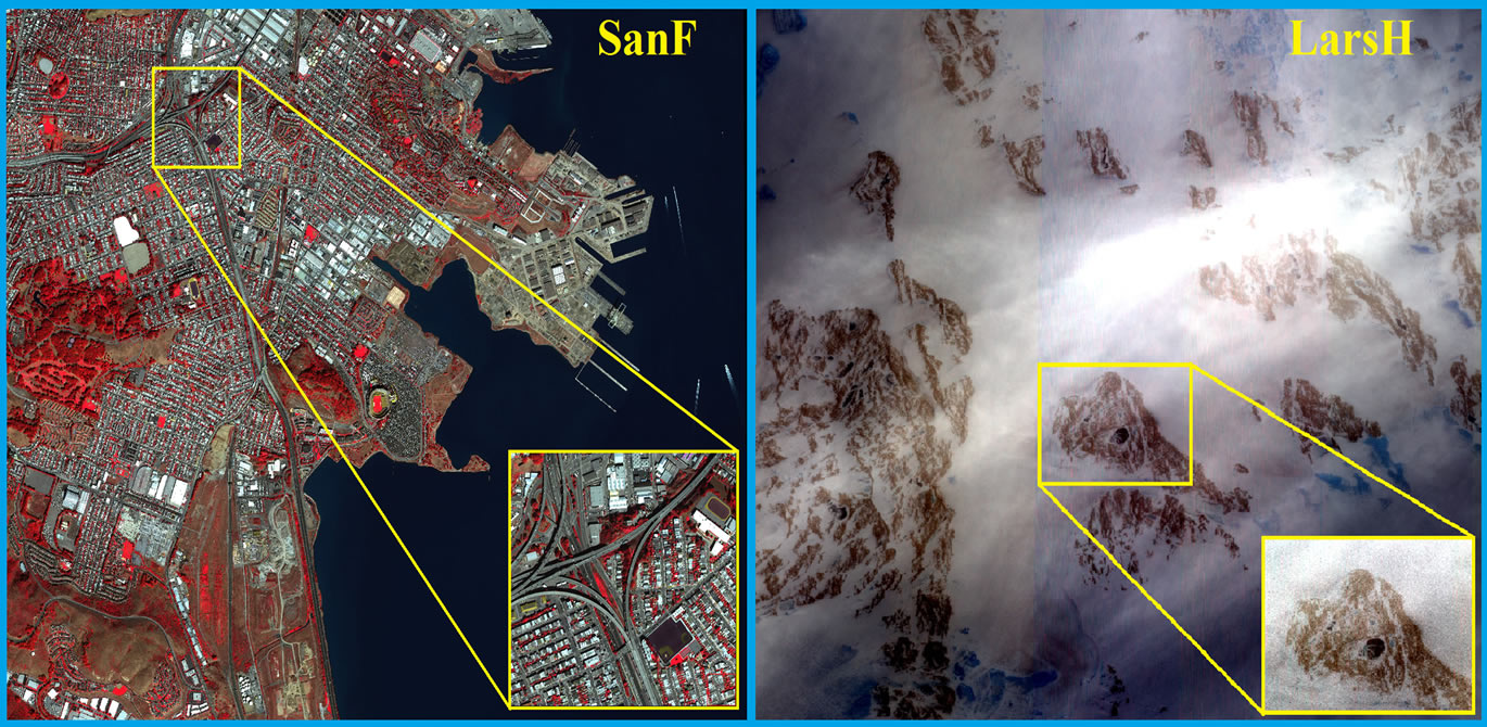
Figure 1. WorldView-2 satellite images highlighting the SanF and LarsH subsets used in present study.
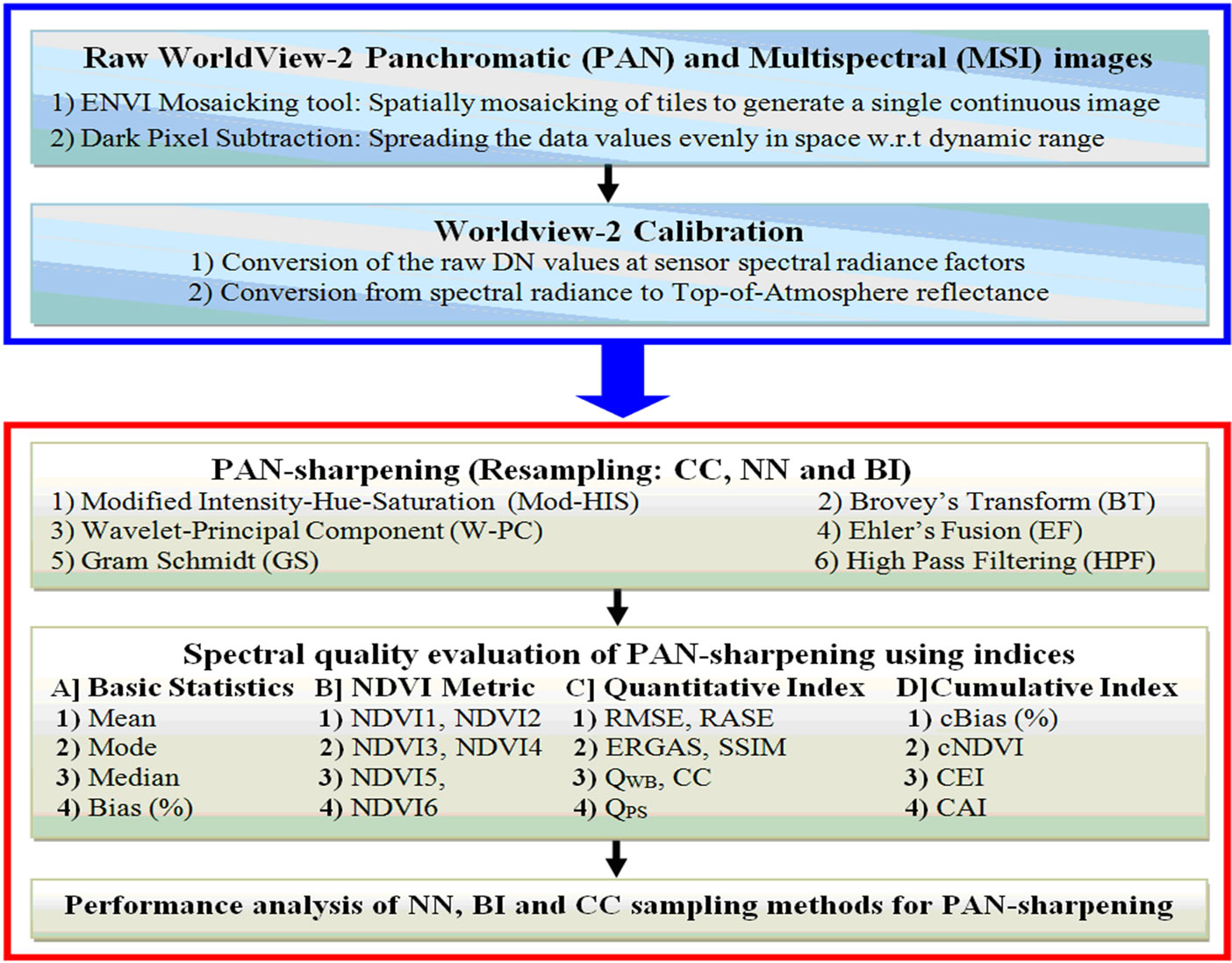
Figure 2. Methodology protocol adapted in the present work.
blocks: 1) data pre-processing, 2) PAN-sharpening with CC, NN, and BI resampling methods, and 3) evaluation of PAN-sharpening and resampling methods. Each block of the methodology (Figure 2) is discussed as follows.
3.1. Data Pre-Processing
Two procedures were implemented for data preprocessing: (a) dark object subtraction (DOS) and (b) data calibration. First, a dark pixel subtraction was performed in order to evenly spread the data values in space with regard to a dynamic range. The DOS was used to reduce the path radiance from each band. The DN values for DOS per band for the WV-2 image are: (15, 39, 54, 34, 54, 37, 89, and 45). Second, the calibration information in a metadata file of the WV-2 imagery was used to calibrate WV-2 by applying the WorldView calibration utility (ENVI 4.8). This calibration method was adapted from the literature [23].
3.2. PAN-Sharpening with CC, NN and BI Resampling Methods
In the present study, the PAN and MSI are captured at the same time with the same sensor. Hence, PANsharpening was carried out directly without further registration. We analyzed PAN-sharpened images after separately applying the chosen resampling methods. There are many resampling methods available for practical use in PAN-sharpening, but each one has trade-offs. A few resampling methods preserve the spectral integrity of the data but may introduce spatial discontinuities in the images, while others have good spatial properties but the spectral values are distorted, especially around sharp edges. Hence, resampling methods should be tested for post-sharpening spectral distortions. In the present study, we have applied NN, CC, and BI resampling methods to determine their effects on the six PAN-sharpening methods—BT, W-PC, EF, GS, Mod-HIS and HPF—on WV-2 datasets and assessed the quality of the sharpened products. These methods were chosen because they cause less spectral distortion than other sharpening methods, such as HIS, PCA, and wavelet transforms [24,25]. After PAN-sharpening, the quality of the sharpened product is examined visually. The visual analysis is based on a visual comparison of colour between the original MSI and the sharpened image and a visual comparison of the spatial details between the original PAN and the sharpened image.
3.3. Statistical Evaluation of PAN-Sharpening Methods
Because the performance of PAN-sharpening algorithms is spectrally and spatially dependent, the spectral and spatial quality of the PAN-sharpened images was evaluated using quality indices. The accuracy statistics for sharpened images were calculated using IDL-7 and Matlab-4 routines [26-31]. In this work, we employed three categories of evaluation indices to compare PAN-sharpening methods: basic statistical parameters, normalized difference vegetation index (NDVI), and quantitative evaluation indices. These evaluation indices include percentage bias [32], NDVI [33], Wang-Bovik index (QWB) [34], structure similarity index (SSIM) [35], root mean square error (RMSE), relative dimensionless global error in synthesis (Erreur Relative Globale Adimensionnelle de Synthese, ERGAS) [36], quality of PAN-sharpening (QPS) [37], relative average spectral error (RASE) and Zhou’s spatial correlation index/high-pass correlation coefficient (HCC) [38,39]. In addition, we introduced a fourth category of evaluation index to evaluate PANsharpening by cumulatively summarizing the quantitative evaluation indices. These cumulative evaluation indices are cumulative NDVI (cNDVI), cumulative bias (cBias), cumulative accuracy index (CAI), and cumulative error index (CEI). The mathematical expressions of these indices are summarized in Tables 1 and 2.
4. Results and Discussion
In the first step of our protocol, productivity, performance ability, and worthiness of the six PAN-sharpening techniques for high-resolution RS images from WV-2 were evaluated visually and quantitatively using four types of quality indices. In the second step, three resampling methods were evaluated for their practical use in the process of PAN-sharpening WV-2 data. To illustrate our research findings, we describe subsets of the WV-2 images based on their location of origin (SanF and LarsH), because each location contains different classes of land-cover. Figure 3 depicts the original MSI (RGB = band 7; band 5; band 3) and the PAN image along with six sharpened images for the SanF subset. The main setback in PAN-sharpening is colour distortion. Hence, colour preservation is the most important criterion in evaluating the performance of sharpening on the basis of visual interpretation. Visual analysis of Figure 3 shows that the colours in the GS, EF, and W-PC sharpened images are similar to the colours in the MSI, which indicates that colours are mostly preserved under the same display conditions. The GS, EF, and W-PC images also show enhanced brightness than BT, Mod-HIS, and HPF, making them more suitable for land-cover classification. Colours in HPF-sharpened images are slightly shallow in tone, while BT-sharpened images show colours with a slightly deep tone. Mod-HIS sharpening results in enhanced red and blue colours. Overall, under the same display conditions, visual analysis shows that the MSI colours are more or less well preserved in all six PAN-
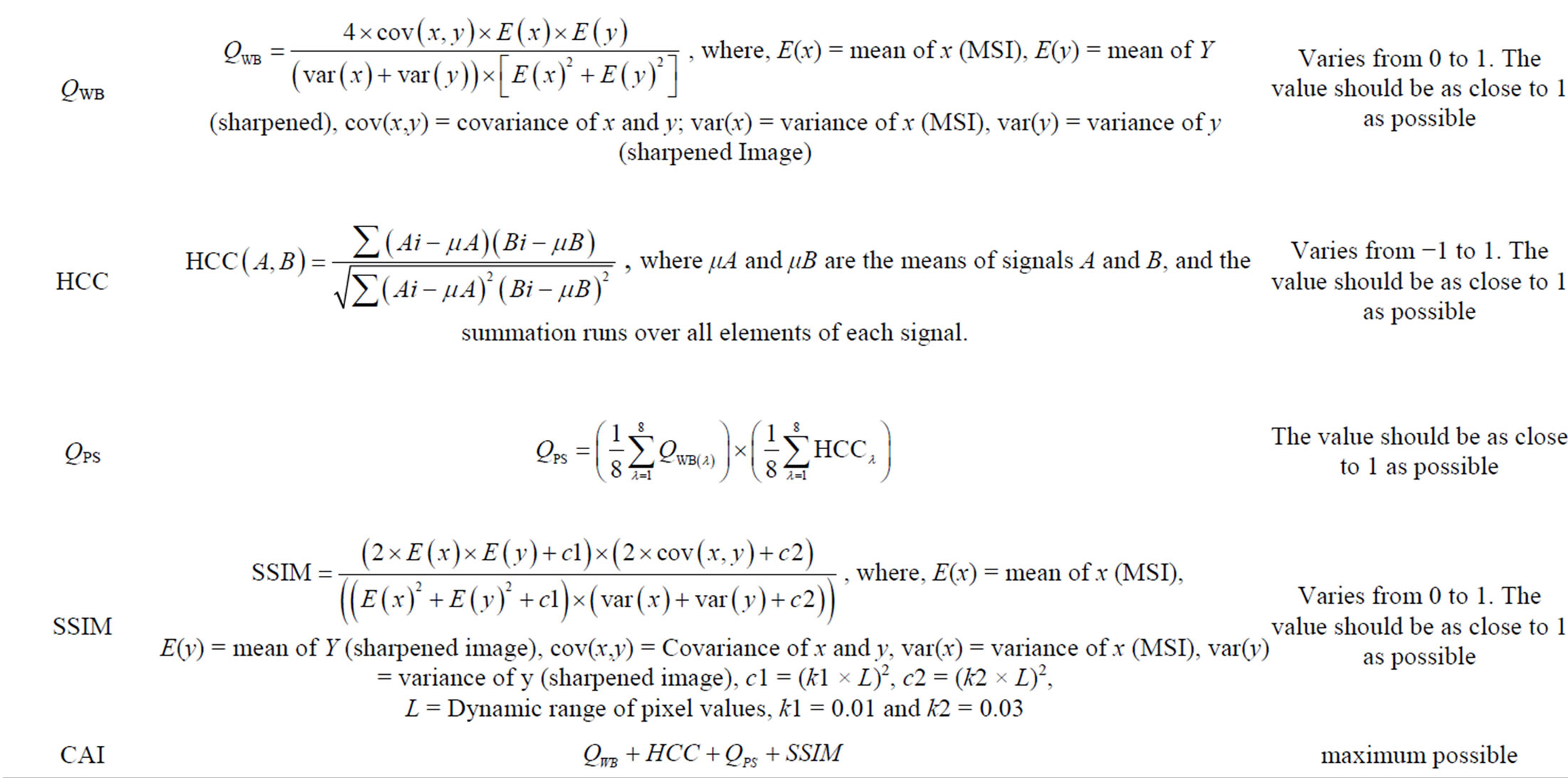
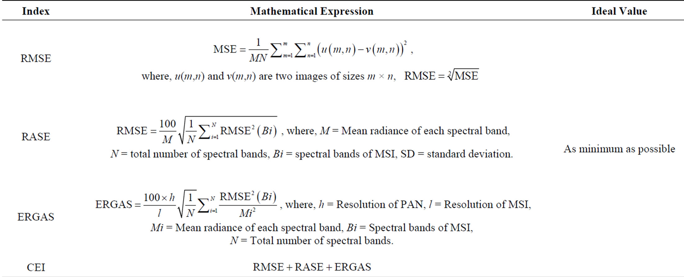
Table 1. Mathematical expressions for quantitative indices for PAN-sharpening quality evaluation.
sharpening methods examined.
4.1. Evaluation of PAN-Sharpening Methods Using Quality Indices
Assessing the quality of PAN-sharpened MS images is an openly debated topic [40]. Many methods are available to evaluate both the spectral and spatial quality of PAN-sharpened images, but there is currently no consensus in the literature regarding which quality index is the best. We used four categories of quality indices to evaluate the quality of PAN-sharpened images, which allowed us to take all the study variables into consideration: 1) three different resampling methods, 2) 20 PANsharpening evaluation indices, and 3) six different PANsharpening methods.
4.1.1. Basic Statistical Indices
The bias (%) in the mean value (also for mode and median) between sharpened and original MSI indicates the percentage by which the mean (median and mode) of the histogram has shifted due to PAN-sharpening.
Specifically, bias quantifies the changes in an image’s histogram caused by the PAN-sharpening process. A positive bias value indicates a shift to white, while a negative value indicates a shift to grey. The bias values (%) in mean, mode, and median for the six PAN-sharpening methods are shown in Table 3. It is evident from Table 3 that the GS process performs best, with the smallest average bias (mean = 0.0929, median = 0.1722, and mode = –0.7391), while the BT performs the worst, with highest average bias (mean = –14.7830, median =
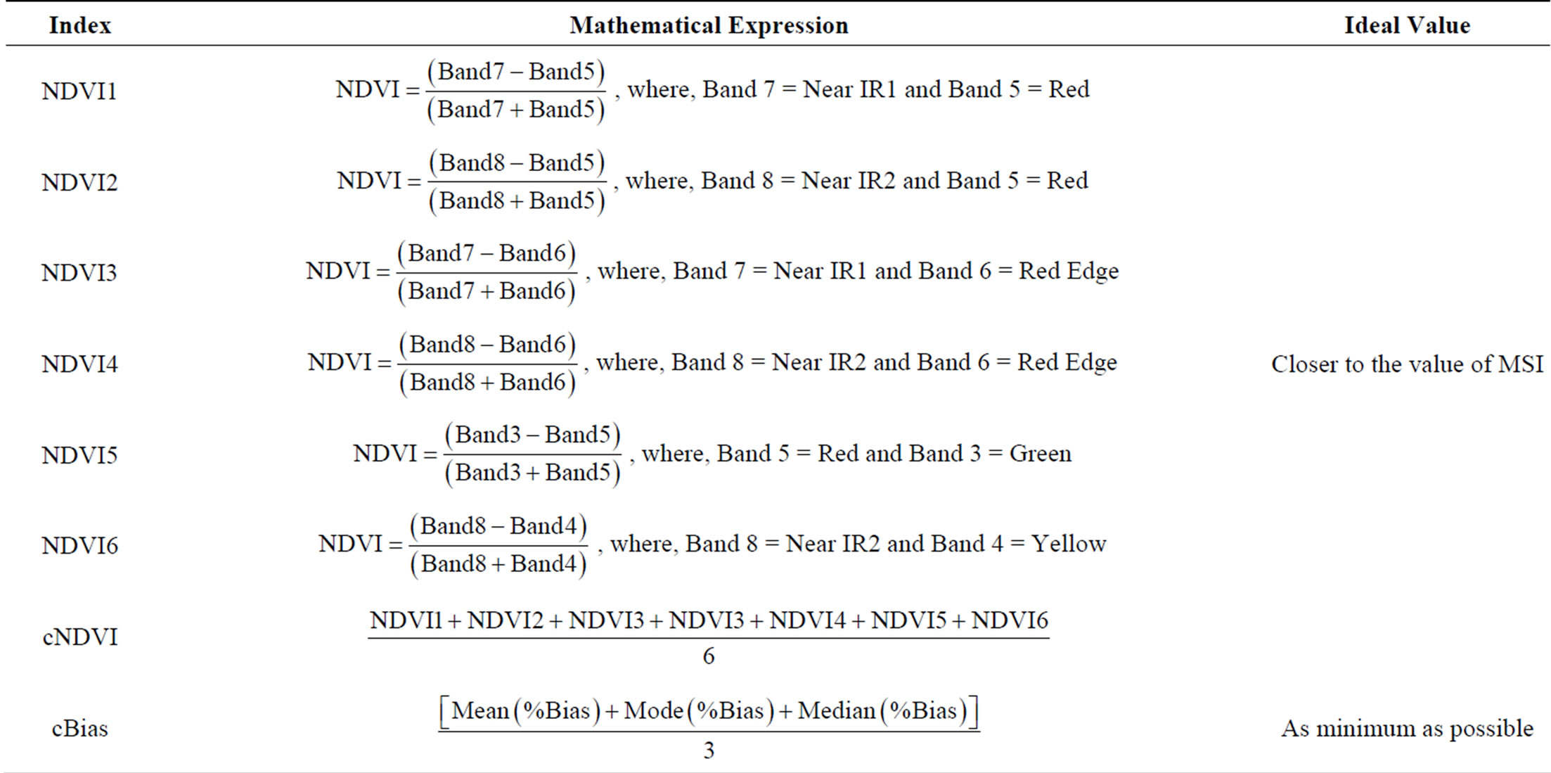
Table 2. Mathematical expressions for quantitative indices for PAN-sharpening quality evaluation.
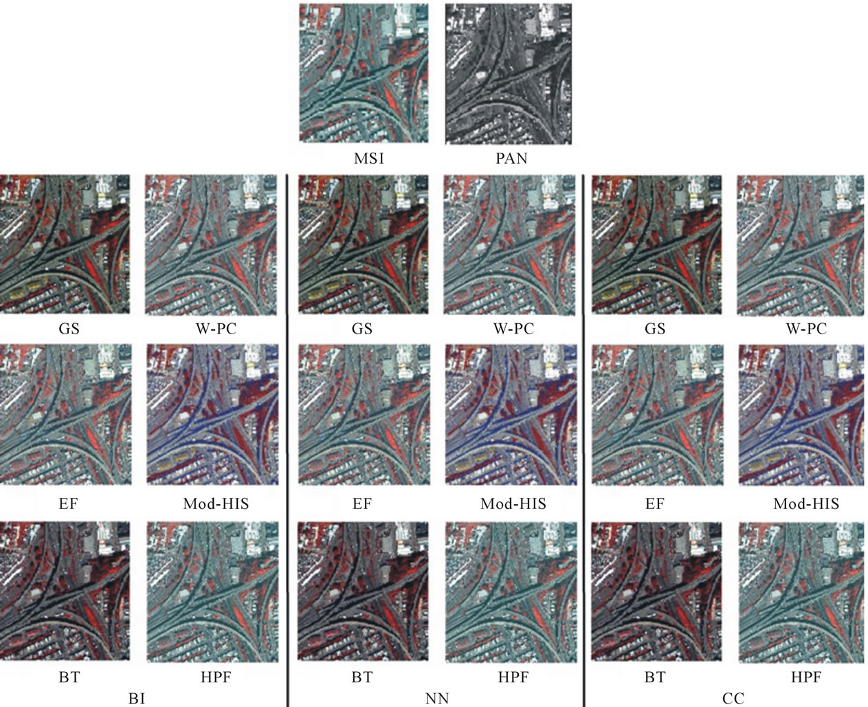
Figure 3. Six PAN-sharpened images of SanF subset using NN (nearest neighbourhood), BI (bilinear interpolation) and CC (cubic convolution) resampling methods.
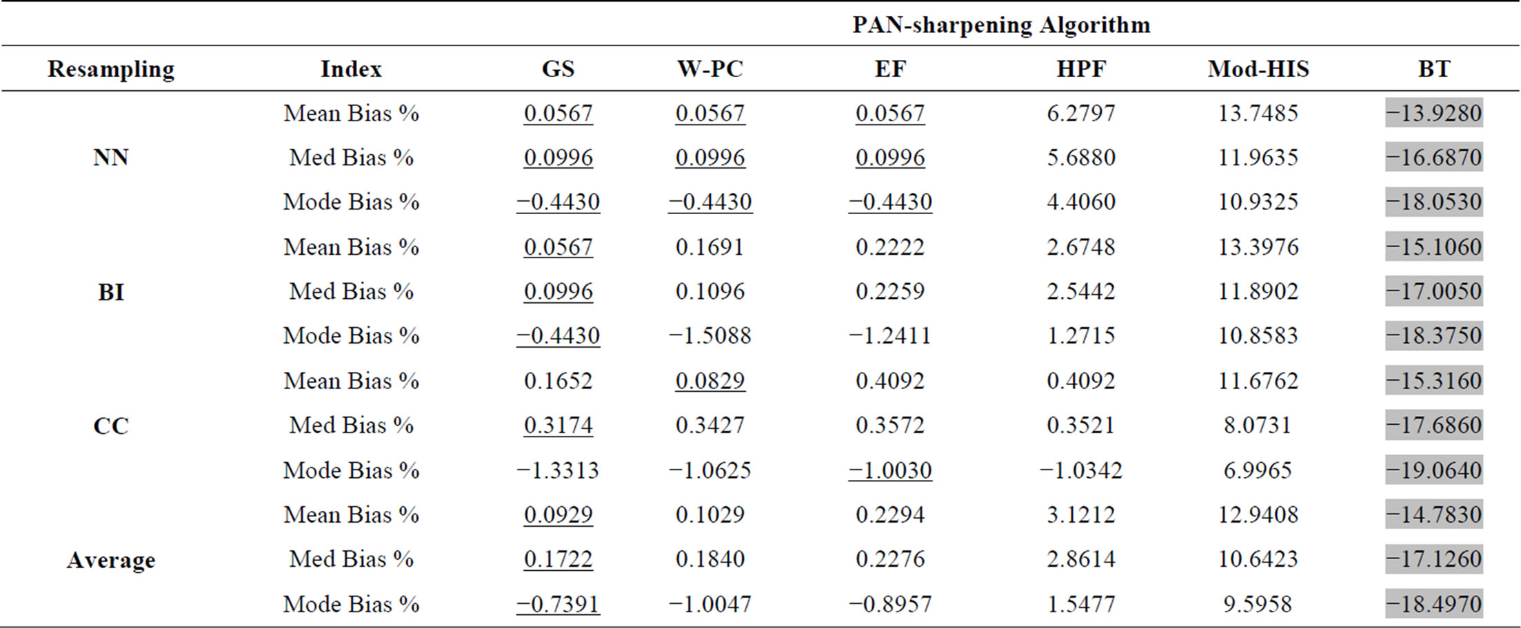
Table 3. Performance of six PAN-sharpening methods evaluated using three basic statistical indices. Row-wise superior (inferior) PAN-sharpening method is underlined (grey).
–17.1260, and mode= –18.4970). All bias values for BT method are negative, indicating that the BT method causes the histogram to shift towards the grey values at higher magnitudes than the other PAN-sharpening methods in the cohort. The EF method performs better than W-PC in terms of mode bias, but W-PC performs better than EF in terms of median bias. The generalized order of performance of PAN-sharpening methods based on the three basic statistical indices can be summarized as: GS > (W-PC = EF) > HPF > Mod-HIS > BT.
From Table 3, it can also be inferred that the mean bias value is much more sensitive to the sharpening effects than the median bias or mode bias, suggesting that the mean bias value is the best statistical indicator to use when evaluating PAN-sharpening methods.
4.1.2. NDVI
These indices quantify variations in the NDVI value because of any pre-processing such as PAN-sharpening. High correlation between the NDVI values from original MSI and the sharpened image indicates less spectral distortion due to PAN-sharpening, i.e., good spectral quality. In the present study, the traditional NDVI formula was modified for 8-band WV-2 data. Since there are duplets of near-IR and red bands, we used six NDVI mathematical expressions to quantify spectral distortions resulting from PAN-sharpening. The statistics in Table 4 indicate that the overall NDVI values for the GS sharpened image are closer to the MSI (correlation = 0.9999), than MSI correlations for other PAN-sharpening algorithms in the study cohort, indicating that the GS method results in the least amount of spectral distortion. The W-PC and EF methods have the same constant average correlation values of 0.9996, while the HPF and Mod-HIS methods have the same correlation values of 0.9997, slightly better than observed for the W-PC and EF methods. Interestingly, the W-PC and EF methods outperformed the HPF and Mod-HIS methods when the algorithms were evaluated using basic statistical indices. The BT method had the lowest correlation coefficient, at 0.9966, indicating that this method causes the greatest amount of spectral distortion in all of the PAN-sharpening methods analyzed. The most surprising observation in the NDVIbased PAN-sharpening analysis was that each of the six NDVI mathematical expressions used resulted in a different performance trend for the PAN-sharpening methods. These discrepancies suggest that the performance of PAN-sharpening, when evaluated using NDVI, dependent on the specific bands used in the NDVI formula. This theory suggests that different WV-2 bands are prone to different degrees of spectral distortion as a result of PAN-sharpening. The performance of PAN-sharpening methods using NDVI is ranked as (best to worst) GS > (HPF = Mod-HIS) > (W-PC = EF) > BT.
4.1.3. Quantitative Indices
The evaluation of PAN-sharpening methods using quantitative indices is shown in Table 5. The statistics in Table 5 suggest that GS sharpened images tend to have the least spectral-spatial distortion than the other PANsharpening methods examined in this study. The GS algorithm is the sharpest algorithm (highest average score), which retained the spectral (QWB = 0.957) and spatial (HCC = 0.985) qualities much better than other PANsharpening algorithms, while the BT algorithm scored the lowest among the six algorithms (QWB = 0.694, HCC = 0.797). In brief, this analysis of quality indices indicates that the GS algorithm maintained the best balance
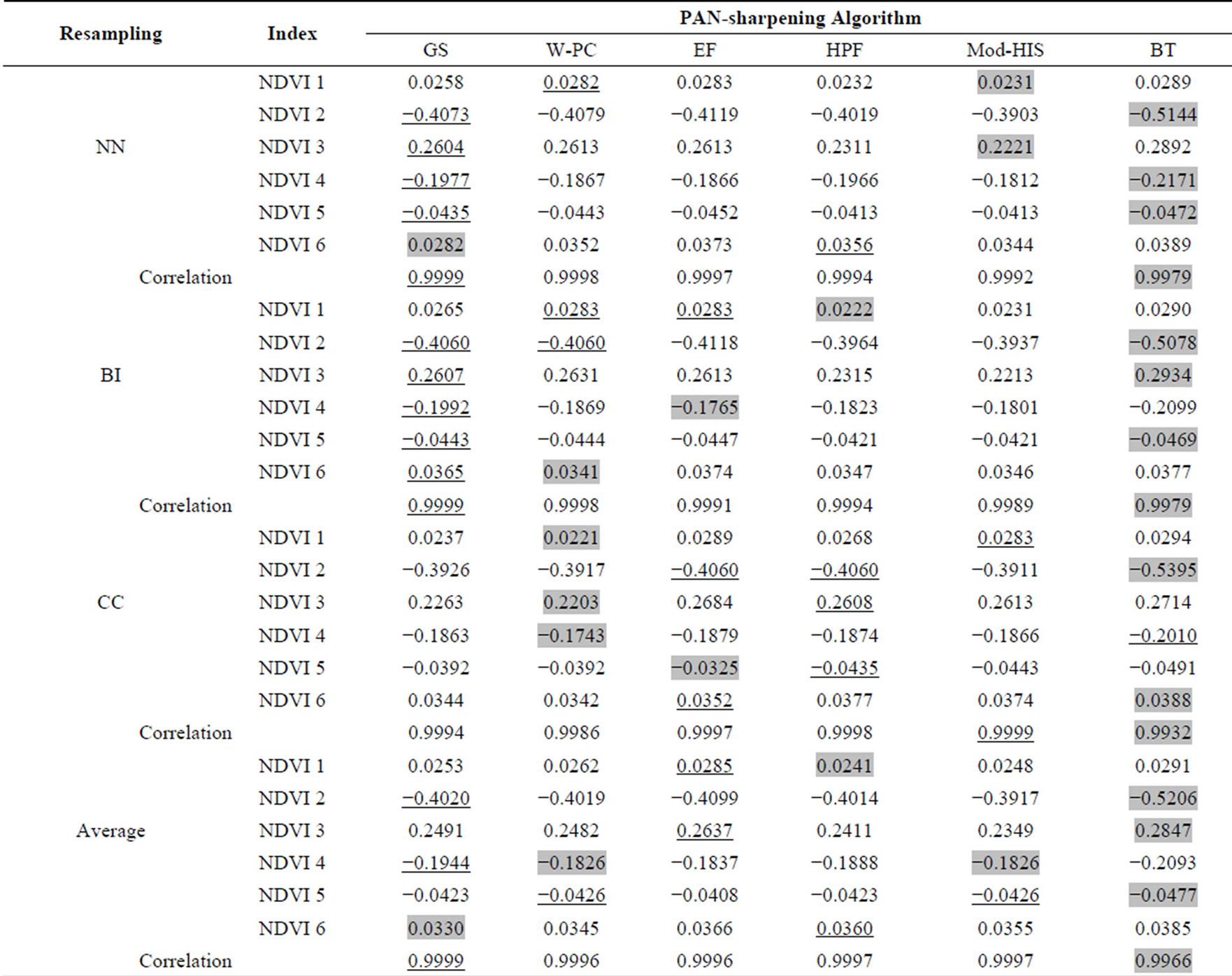
Table 4. Performance based ranking/trend for six PAN-sharpening methods evaluated using six NDVI metrics. Superior (inferior) PAN-sharpening methods are underlined (grey).
between spectral and spatial quality and therefore outperformed the other PAN-sharpening algorithms. The variations in quantitative indices for different PANsharpened images can be attributed to the varying spectral and/or spatial distortions caused by PAN-sharpening processing. Table 5 shows that the smallest average error values are found when the GS method is used (RMSE = 28.9519, RASE = 4.8147, and ERGAS = 1.1690), followed by the W-PC method (RMSE = 32.3346, RASE = 5.3911, and ERGAS = 1.3064), and then the EF method (RMSE = 36.2186, RASE = 6.0503, and ERGAS = 1.5586). The highest accuracy values are found when the GS method is used (QWB = 0.957, QPS = 0.9423, and SSIM = 0.8100), again followed by W-PC method (QWB = 0.847, QPS = 0.8417, and SSIM = 0.8067). As for the RMSE, RASE and ERGAS values, GS, W-PC, and EF sharpened images showed smaller error values than the other methods. In general, in terms of quantitative evaluation indices, we can conclude that the GS method shows the best spectral and spatial performances, whereas the W-PC and EF approaches occasionally lead to similar results. The spectral and spatial performances of PAN-sharpening algorithms can be ranked quantitatively in terms of RASE, RMSE, QWB, SSIM, ERGAS, HCC and QPS (Table 5), resulting in the performance trend of GS > W-PC > EF > HPF > Mod-HIS > BT. This trend indicates that the GS algorithm outperformed and the BT algorithm underperformed the other PAN-sharpening algorithms tested.
However, we note that the values of ERGAS, HCC, SSIM and QWB for W-PC and GS are comparable due to the fact that GS algorithm models the input bands in a slightly better fashion than W-PC. This is evident from the individual spectral quality (RMSE, RASE and ERGAS) and spatial quality (QPS) values for GS and W-PC algorithms. We note that the variations in all the quantitative evaluation indices for six PAN-sharpening methods are comparable, indicating that differences were
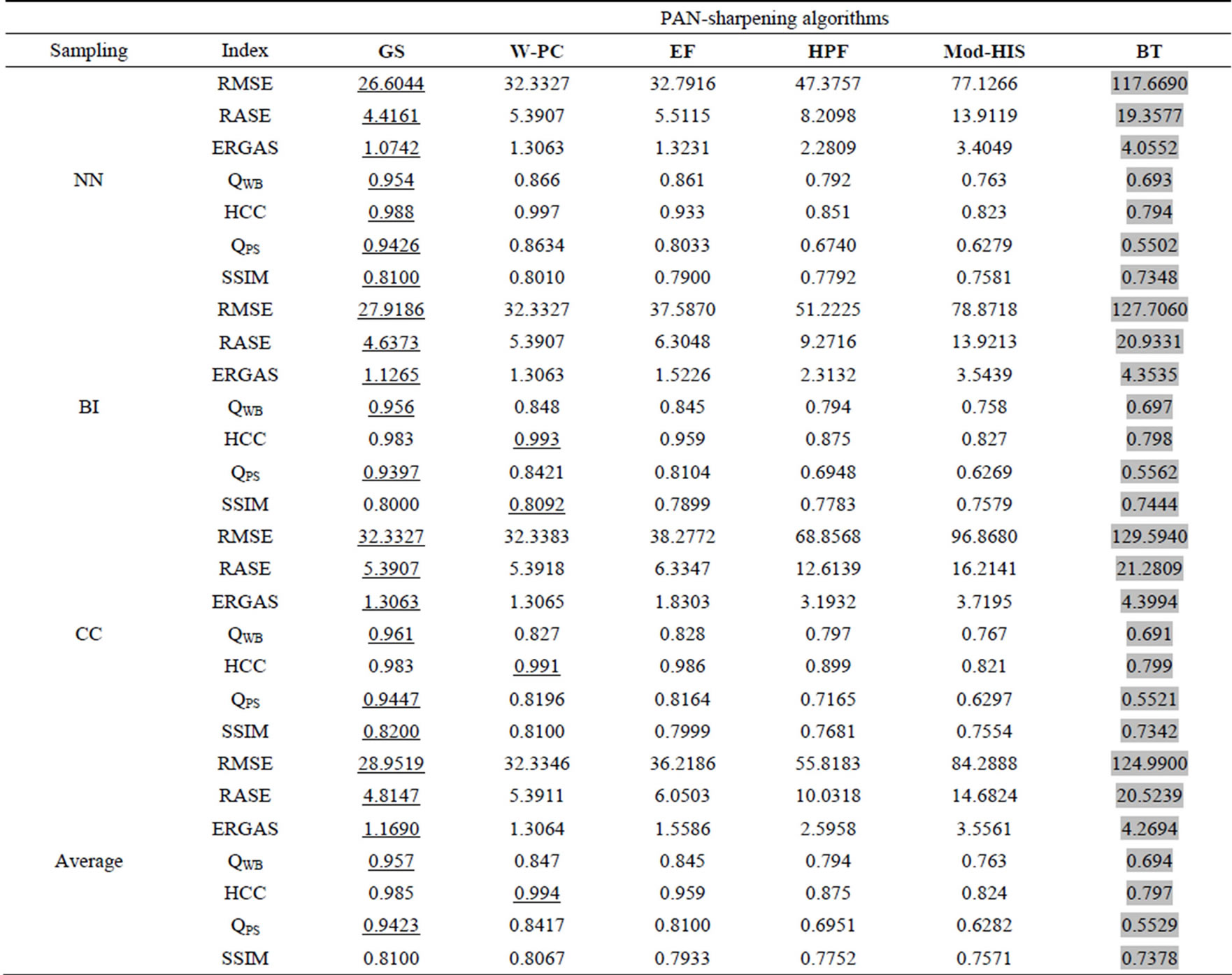
Table 5. Performance based trend for six PAN-sharpening methods evaluated using seven quantitative indices. Row-wise superior PAN-sharpening method is underlined while inferior one is highlighted in grey.
not caused by variation in either spectral or spatial quality, but arose because of the overall performance (both spatial and spectral quality) of the algorithm. The PANsharpening methods using the HCC index, which represents spatial quality, can be ranked according to the performance as: W-PC > GS > EF > HPF > Mod-HIS > BT. In this trend, W-PC performed better than GS. This contrasts the trend found when spectral qualities (QWB) were used to rank performance, in which GS performed better than W-PC. These findings indicate that between GS and W-PC algorithms, there is a trade-off between spatial quality and spectral quality. In other words, the trend suggests that for the GS method, the poor spatial performance was offset by the excellent spectral performance, and vice-versa for the W-PC method. The spectral and spatial qualities are interdependent for these two PAN-sharpening algorithms. Interestingly, all of the quantitative indices allowed for a clear comparison between PAN-sharpening methods, even more so than the other evaluation indices, namely basic statistical indices and NDVI indices.
4.1.4. Cumulative Indices
For the last group of evaluation indices, we developed a set of cumulative indices to summarize the results from the three PAN-sharpening evaluation approaches, the basic statistical approach, the NDVI approach, and the quantitative evaluation approach. The results of analyzing PAN-sharpening methods by using the cumulative indices are shown in Table 6. It shows the performance trends of the PAN-sharpening algorithms based on cBias, cNDVI, CAI, and CEI values. It is evident from Table 6 that the GS method outperformed other methods, attaining the lowest average CEI (34.9356) and the highest CAI (3.6940) scores. Conversely, BT had the worst performance, achieving the highest CEI (149.7830) and the lowest CAI (2.7813) scores of the PAN-sharpening methods analyzed. The performance trend of PAN-
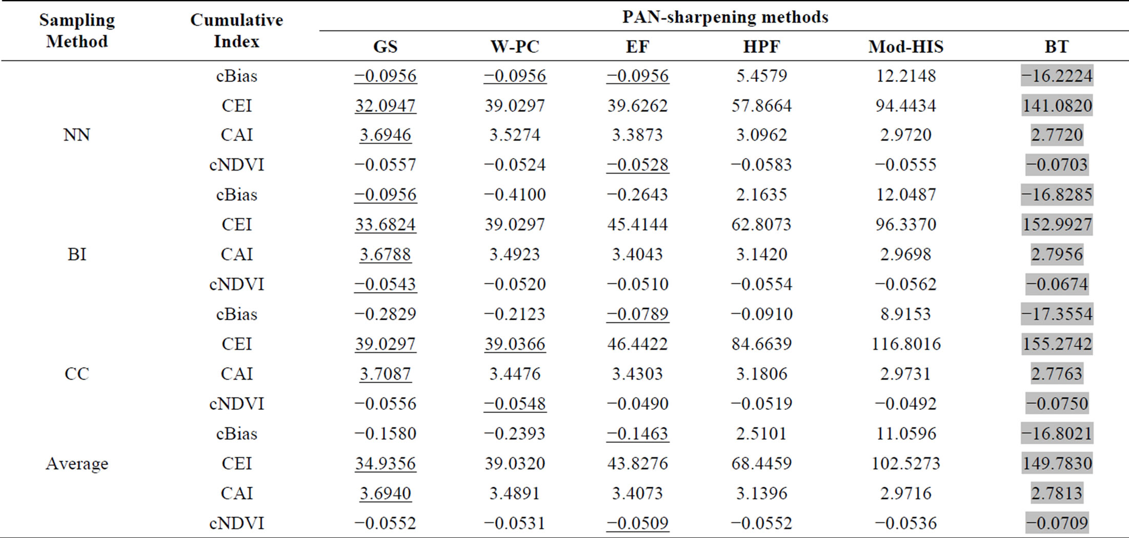
Table 6. Performance based trend for six PAN-sharpening methods evaluated using four cumulative indices. Row-wise superior (inferior) PAN-sharpening method is underlined (grey).
sharpening methods using the CAI and CEI indices shows GS > W-PC > EF > HPF > Mod-HIS > BT.
However, when using the other cumulative indices, we found different results. The EF method performed the best with respect to the cBias (–0.1463) and cNDVI (–0.0509) indices. The performance trend when applying the cBias index is EF > GS > W-PC > HPF > Mod-HIS > BT, while the performance trend when using cNDVI is EF > W-PC > Mod-HIS > (HPF = GS) > BT. Table 6 shows that the CAI and CEI indices are much more sensitive to a method’s sharpening effects than the cNDVI and cBias indices, suggesting that the CAI and CEI values may be the best statistical indicators to evaluate PAN-sharpening methods. One possible reason for the variations in performance trends seen when using cBias and cNDVI may be that six different variants of NDVI were used to formulate the cNDVI index and three different statistical indices (mean, mode and median) were used to derive the cBias index.
4.2. Evaluation of Resampling Methods for PAN-Sharpening WV-2 Data
As discussed earlier, the resampling method used in PAN-sharpening processes can cause varying amounts of spectral distortions depending on the PAN-sharpening algorithms used. Therefore it is necessary to evaluate the practicability of different resampling methods in order to produce superior PAN-sharpening results. Because PANsharpening affects the final classification process, evaluating different resampling methods to select the best one for a particular PAN-sharpening algorithm is necessary to reduce potential classification errors. The main way to visually analyze PAN-sharpening methods is by observing distortions in colour. A visual analysis of Figure 3 shows that the colours of all PAN-sharpened images resampled with NN, CC, and BI methods are comparable to the MSI, which suggests that the colour is mostly preserved when images are displayed under the same conditions, even when different resampling methods are used.
4.2.1. Basic Statistical Indices
Performance results of the resampling methods evaluated using basic statistical indices are presented in Table 3. The statistics in Table 3 show that the NN resampling method performed best for the GS, EF, BT, and W-PC sharpening methods, while CC performed well for the HPF and Mod-HIS methods. Interestingly, the NN resampling method proved poor for the HPF and Mod-HIS methods, while the CC resampling method was inferior when used with the GS, BT, and EF methods, but performed moderately when paired with the W-PC methods. Surprisingly, the performances of the BI and NN resampling methods were almost equivalent when used with the GS sharpening method. The overall performance of the BI resampling method was moderate when used with any of the PAN-sharpening methods. Based on these observations, the overall performance trend of resampling methods when evaluated by basic statistical indices was NN > BI > CC. For the GS, EF, BT, and W-PC PAN-sharpening methods, the performance trend remained NN > BI > CC, but for the HPF and Mod-HIS methods, the trend was CC > BI > NN. In general, using basic statistical indices, we conclude that the NN resampling method exhibits superior performance over CC and BI resampling methods because it causes less spectral distortion of PAN-sharpened WV-2 images.
4.2.2. NDVI
Performance results of resampling methods evaluated by six NDVIs are shown in Table 4. The statistics in Table 4 indicate that the NN and BI resampling methods performed best with GS and W-PC methods, while CC performed well with HPF and Mod-HIS methods. For the BT PAN-sharpening method, the CC and BI resampling methods well, while NN performed moderately. From Table 4, we observe that the CC and NN resampling methods performed well for all PAN-sharpening methods evaluated by NDVIs with positive values (NDVI1, NDVI3, and NDVI6), while BI performed moderately in terms of these same positively valued NDVIs. On the other hand, BI and CC resampling methods performed well for all PAN-sharpening methods evaluated by NDVIs with negative values (NDVI2, NDVI4, and NDVI5), while NN performed moderately in terms of these negatively valued NDVIs. With respect to the GS and W-PC sharpening algorithms, the performances of BI and NN resampling methods were almost equivalent, but the CC resampling method performed poorly. For EF sharpening, the CC method performed best, but the NN and BI resampling methods performed poorly. Overall, the BI resampling method performed moderately with all PAN-sharpening methods.
4.2.3. Quantitative Indices
Performance results of resampling methods evaluated by seven quantitative indices are shown in Table 5. The statistics in Table 5 indicate that for the W-PC, Mod-HIS, and BT sharpening algorithms, the NN and BI resampling methods performed best. For the GS, HPF, and EF sharpening algorithms, the CC and NN resampling methods performed best. From Table 5, we observe that for all PAN-sharpening algorithms the NN resampling method outperformed the other resampling methods when evaluated by the error indices (RMSE, RASE and ERGAS). On the other hand, the CC method performed the best for all PAN-sharpening algorithms when evaluated by the accuracy indices (QWB, HCC, QPS, and SSIM). Based on the quantitative indices, we conclude that the NN and CC resampling methods display the best performance with PAN-sharpening of WV-2 images because they cause the lease amount of spectral distortion.
4.2.4. Cumulative Indices
Performance results of resampling methods evaluated by four cumulative indices are shown in Table 6. The statistics in Table 6 show that the NN and BI resampling methods performed well in conjunction with the GS, W-PC, and BT algorithms, while CC and NN performed best with the HPF, EF, and Mod-HIS algorithms. It was also found that for all PAN-sharpening algorithms, the NN method performed the best when using the using CEI, while BI performed moderately and CC performed poorly using the CEI. On the other hand for all PANsharpening algorithms, the CC and NN resampling methods performed the best when evaluated using cBias, and BI performed moderately. Furthermore, we found that the CC resampling method performed better with almost all PAN-sharpening methods when the CAI was used for evaluation. With respect to the cNDVI, the BI method performed better than the NN and CC resampling methods for all PAN-sharpening algorithms.
4.3. Practicability of Resampling Methods for Different PAN-Sharpening Algorithms
Based on results from the comprehensive quality evaluation of PAN-sharpened images, we now comment on resampling methods yielding the best performances for individual PAN-sharpening algorithms. The three resampling methods performed similarly for all of the PANsharpening algorithms except the HPF and Mod-HIS algorithms. The performance evaluation indicates that the NN resampling method can be appropriately implemented with GS, W-PC, EF, and BT PAN-sharpening algorithms. On the other hand, the CC resampling method can be implemented with the Mod-HIS and HPF PAN-sharpening algorithms.
5. Conclusion
In this work, the performances of six different PANsharpening algorithms, modified HIS, W-PC, BT, GS, EF and HPF were comprehensively evaluated as a means to fuse WV-2 PAN and MS data. In general, all of the sharpening techniques improve the resulting image resolution and the detection of small targets, like cars, buildings and trees. The GS, EF, and W-PC sharpening algorithms preserve, in general, the original MSI colours in all the possible RGB band combinations. In contrast, the Mod-HIS, BT, and HPF sharpening techniques cause changes in the colours of the original images and make image interpretation more difficult. In terms of statistical indices, our analysis indicated that the GS, W-PC, and EF methods again yield the best results compared to the other methods. For all of the quality indices, the performance trend is almost fully preserved: GS > W-PC > EF > HPF > Mod-HIS > BT. This study did not aim to determine the best method for image resampling, but it focused on how commonly used resampling methods visually and statistically change the PAN-sharpening results. For all six PAN-sharpening algorithms, we did not find any significant colour difference in the sharpened images based on the resampling method used. However, in general, our statistical comparison suggested that the CC resampling method provided poorer results when compared to the NN resampling method. In general, we conclude that the CC resampling method should be used in conjunction with Mod-HIS and HPF PAN-sharpening algorithms, and the NN resampling method should be used in conjunction with the BT, GS, EF, and W-PC PAN-sharpening algorithms. In general, we conclude that the choice of the resampling method does not have any significant visual effect on the PAN-sharpened image, but the sharpened image should be assessed for the statistical changes caused by the chosen resampling method. It is important to carefully select the most appropriate resampling technique for a given sharpening algorithm, and then apply the same resampling technique to all of the images in a remote sensing application. The present analysis has shown that the quality of a PAN-sharpened image is statistically dependent on the choice of the resampling method.
6. Acknowledgements
We are indebted to the organizers of the DigitalGlobe Inc. 8-band Research Challenge (2010-2011) and the IEEE GRSS Data Fusion Data Fusion Contest (2012), who provided the research platform and the necessary images to our research team, free of cost. We acknowledge Dr. Celeste Brennecka for her constructive comments on the draft version of manuscript. The comments from Ms. Stephanie Grebas and Ms. Prachi Vaidya, benefitted the paper. We acknowledge Mr. Rohit Paranjape, Mr. Parag Khopkar and Mr. Sagar Jadhav, for their contribution in initial data processing. We also acknowledge Dr. Rajan, NCAOR Director, and Mr. R. Ravindra, former NCAOR Director, for their encouragement and motivation for this research. This is NCAOR contribution no. 16/2013.
REFERENCES
- Y. Zhang, “Highlight Article: Understanding Image Fusion,” Photogrammetric Engineering & Remote Sensing, Vol. 70, No. 6, 2004, pp. 657-661. http://studio.gge.unb.ca/UNB/zoomview/PERS_Vol70_No6_paper.pdf
- U. Kumar, C. Mukhopadhyay and T. V. Ramachandra, “Pixel Based Fusion Using IKONOS Imagery,” International Journal of Recent Trends in Engineering, Vol. 1, No. 1, 2009, pp. 173-175. http://www.academypublisher.com/ijrte/vol01/no01/ijrte0101173177.pdf
- I. Amro, J. Mateos, M. Vega, R. Molina and A. K. Katsaggelos, “A Survey of Classical Methods and New Trends in Pansharpening of Multispectral Images,” EURASIP Journal on Advances in Signal Processing, Vol. 2011, 2011, p. 79. http://dx.doi.org/10.1186/1687-6180-2011-79
- Q. Du, N. H. Younan, R. King and V. P. Shah, “On the Performance Evaluation of Pan-Sharpening Techniques,” IEEE Geoscience and Remote Sensing Letters, Vol. 4, No. 4, 2007, pp. 518-522.
- M. Choi, “A New Intensity-Hue-Saturation Fusion Approach to Image Fusion with a Tradeoff Parameter,” IEEE Transactions on Geoscience and Remote Sensing, Vol. 44, No. 6, 2006, pp. 1672-1682. http://dx.doi.org/10.1109/TGRS.2006.869923
- U. Kumar, A. Dasgupta, C. Mukhopadhyay, N. V. Joshi and T. V. Ramachandra, “Comparison of 10 Multi-Sensor Image Fusion Paradigms for IKONOS Images,” International Journal of Research and Reviews in Computer Science (IJRRCS), Vol. 2, No. 1, 2011, pp. 40-47. http://www.ces.iisc.ernet.in/energy/paper/ijrrcs_ikonos_fusion/image.htm
- J. Vrabel, P. Doraiswamy, J. McMurtrey and A. Stern, “Demonstration of the Accuracy of Improved Resolution Hyperspectral Imagery,” SPIE Proceedings, Vol. 4725, No. 1, 2002, pp. 556-567. http://dx.doi.org/10.1117/12.478790
- W. A. Hallada and S. Cox, “Image Sharpening for Mixed Spatial and Spectral Resolution Satellite Systems,” Proceedings of the 17th International Symposium on Remote Sensing of Environment, Ann Arbor, 9-13 May 1983, pp. 1023-1032.
- P. Pradhan, R. King, N. H. Younan and D. W. Holcomb, “The Effect of Decomposition Levels in Wavelet-Based Fusion for Multiresolution and Multi-Sensor Images,” IEEE Transactions on Geoscience and Remote Sensing, Vol. 44, No. 12, 2006, pp. 3674-3686. http://dx.doi.org/10.1109/TGRS.2006.881758
- R. A. Schowengerdt, “Reconstruction of Multispatial, Multispectral Image Data Using Spatial Frequency Content,” Photogrammetric Engineering & Remote Sensing, Vol. 46, No. 10, 1980, pp. 1325-1334.
- C. A. Laben, V. Bernard and W. Brower, “Process for Enhancing the Spatial Resolution of Multispectral Imagery Using Pan-Sharpening,” US Patent No. 6011875, 2000.
- L. Alparone, L. Wald, J. Chanussot, P. Gamba and L. M. Bruce, “Comparison of Pansharpening Algorithms: Outcome of the 2006 GRS-S Data-Fusion Contest,” IEEE Transactions on Geoscience and Remote Sensing, Vol. 45, No. 10, 2007, pp. 3012-3021. http://dx.doi.org/10.1109/TGRS.2007.904923
- C. Thomas, T. Ranchin, L. Wald and J. Chanussot, “Synthesis of Multispectral Images to High Spatial Resolution: A Critical Review of Fusion Methods Based on Remote Sensing Physics,” IEEE Transactions on Geoscience and Remote Sensing, Vol. 46, No. 5, 2008, pp. 1301-1312. http://dx.doi.org/10.1109/TGRS.2007.912448
- F. Van Der Meer, “What Does Multisensor Image Fusion Add in Terms of Information Content for Visual Interpretation?” International Journal of Remote Sensing, Vol. 18, No. 2, 1997, pp. 445-452. http://dx.doi.org/10.1080/014311697219187
- Y. Zhang, “A New Merging Method and Its Spectral and Spatial Effects,” International Journal of Remote Sensing, Vol. 20, No. 10, 1999, pp. 2003-2014. http://dx.doi.org/10.1080/014311699212317
- L. Wald, T. Ranchin and M. Mangolini, “Fusion of Satellite Images of Different Spatial Resolutions: Assessing the Quality of Resulting Images,” PE & RS, Vol. 63, No. 6, 1997, pp. 691-699.
- S. Li, Z. Li and J. Gong, “Multivariate Statistical of Measures for Assessing the Quality of Image Fusion,” International Journal of Image and Data Fusion, Vol. 1, No. 1, 2010, pp. 47-66. http://dx.doi.org/10.1080/19479830903562009
- C. Pohl and J. L. Van Genderen, “Multi-Sensor Image Fusion in Remote Sensing: Concepts, Methods, and Applications,” International Journal of Remote Sensing, Vol. 19, No. 4, 1998, pp. 743-757.
- R. Keys, “Cubic Convolution Interpolation for Digital Image Processing,” IEEE Transactions on Signal Processing, Acoustics, Speech, and Signal Processing, Vol. 29, No. 6, 1981, pp. 1153-1160. http://dx.doi.org/10.1109/TASSP.1981.1163711
- D. L. Verbyla, “Practical GIS Analysis,” Taylor & Francis, London, 2002. http://dx.doi.org/10.1201/9780203217931
- J. A. Parker, R. V. Kenyon and D. E. Troxel, “Comparison of Interpolating Methods for Image Resampling,” IEEE Transactions on Medical Imaging, Vol. 2, No.1, 1983, pp. 31-39, http://dx.doi.org/10.1109/TMI.1983.4307610
- T. M. Lehmann, C. Gonner and K. Spitzer, “Survey: Interpolation Methods in Medical Image Processin,” IEEE Transactions on Medical Imaging, Vol. 18, No. 11, 1999, pp. 1049-1075. http://dx.doi.org/10.1109/42.816070
- T. Updike and C. Comp, “Radiometric Use of WorldView-2 Imagery,” Technical Note, DigitalGlobe®, Colorado, 2010. www.digitalglobe.com/downloads/Radiometric_Use_of_WorldView-2_Imagery.pdf
- T.-M. Tu, S.-C. Su, H.-C. Shyu and P. S. Huang, “A New Look at HIS-Like Image Fusion Methods,” Information Fusion, Vol. 2, No. 3, 2001, pp. 177-186. http://dx.doi.org/10.1016/S1566-2535(01)00036-7
- Y. Zhang, “Problems in the Fusion of Commercial HighResolution Satellites Images as well as LANDSAT 7 Images and Initial Solutions,” International Archives of Photogrammetry and Remote Sensing, Vol. 34, No. 4, 2002.
- S. D. Jawak and A. J. Luis, “Applications of WorldView-2 Satellite Data for Extraction of Polar Spatial Information and DEM of Larsemann Hills, East Antarctica,” Proceedings of International Conference on Fuzzy Systems and Neural Computing, Vol. 2, IEEE, Hong Kong, 2011, pp. 148-151.
- S. D. Jawak and A. J. Luis, “WorldView-2 Satellite Remote Sensing Data for Polar Geospatial Information Mining of Larsemann Hills, East Antarctica,” Proceedings of 11th Pacific (Pan) Ocean Remote Sensing Conference (PORSEC), Kochi, 5-9 November 2012.
- S. D. Jawak and A. J. Luis, “High Resolution 8-Band WorldView-2 Satellite Remote Sensing Data for Polar Geospatial Information Mining and Thematic Elevation Mapping of Larsemann Hills, East Antarctica,” 11th International Symposium on Antarctic Earth Sciences (ISAES XI), Edinburgh, 10-15 July 2011, p. 187.
- S. D. Jawak and A. J. Luis, “Hyperspatial WorldView-2 Satellite Remote Sensing Data for Polar Geospatial Information Mining of Larsemann Hills, East Antarctica,” XXXII SCAR OSC, Portland, 2012.
- S. D. Jawak and A. J. Luis, “A Spectral Index RatioBased Antarctic Land-Cover Mapping Using Hyperspatial 8-Band WorldView-2 Imagery,” Polar Science, Vol. 7, No. 1, 2013, pp. 18-38. http://dx.doi.org/10.1016/j.polar.2012.12.002
- S. D. Jawak and A. J. Luis, “Improved Land Cover Mapping Using High Resolution Multiangle 8-Band Worldview-2 Satellite Remote Sensing Data,” Journal of Applied Remote Sensing, Vol. 7, No. 1, 2013, Article ID: 073573. http://dx.doi.org/10.1117/1.JRS.7.073573
- V. Vijayaraj, N. Younan and C. G. O’Hara, “Concepts of Image Fusion in Remote Sensing Application,” IEEE International Conference on Geoscience and Remote Sensing Symposium, Vol. 10, No. 6, 2006, pp. 3781-3784. http://dx.doi.org/10.1109/IGARSS.2006.973
- V. Vijayaraj, N. Younan and C. G. O’Hara, “Quantitative Analysis of Pansharpened Images,” Optical Engineering, Vol. 45, No. 4, 2004, Article ID: 046202. http://dx.doi.org/10.1117/1.2195987
- Z. Wang and A. C. Bovik, “Universal Image Quality Index,” IEEE Signal Processing Letters, Vol. 9, No. 3, 2002, pp. 81-84. http://dx.doi.org/10.1109/97.995823
- Z. Wang, A. C. Bovik, H. R. Sheikh and E. P. Simoncelli, “Image Quality Assessment: From Error Visibility to Structural Similarity,” IEEE Transactions on Image Processing, Vol. 13, No. 4, 2004, pp. 600-612. http://dx.doi.org/10.1109/TIP.2003.819861
- L. Wald, “Quality of High Resolution Synthesised Images: Is There a Simple Criterion?” Proceedings of the Third Conference “Fusion of Earth Data: Merging Point Measurements, Raster Maps and Remotely Sensed Images”, Sophia Antipolis, 26-28 January 2000, pp. 99-103.
- C. Padwick, M. Deskevich, F. Pacifici and S. Smallwood, “WorldView 2 Pan-Sharpening,” ASPRS Annual Conference, San Diego, 26-30 April 2010.
- J. Zhou, D. L. Civco and J. A. Silander, “A Wavelet Transform Method to Merge Landsat TM and SPOT Panchromatic Data,” International Journal of Remote Sensing, Vol. 19, No. 4, 1998, pp. 743-757. http://dx.doi.org/10.1080/014311698215973
- Y. Zhang, “Methods for Image Fusion Quality Assessment —A Review, Comparison and Analysis,” The International Archives of the Photogrammetry, Remote Sensing and Spatial Information Sciences, Vol. 37, Pt. B7, 2008, pp. 1101-1110.
- C. Thomas and L. Wald, “Assessment of the Quality of Fused Products,” 24th EARSeL Symposium “New Strategies for European Remote Sensing”, Dubrovnik, 25-27 May 2005, pp. 317-325.