Advances in Computed Tomography
Vol.2 No.2(2013), Article ID:33353,8 pages DOI:10.4236/act.2013.22013
Modified Maximum Likelihood Estimation of the Spatial Resolution for the Elliptical Gamma Camera SPECT Imaging Using Binary Inhomogeneous Markov Random Fields Models
Department of Statistics and Actuarial-Financial Mathematics, University of the Aegean, Karlovassi, Greece
Email: zimste@aegean
Copyright © 2013 Stelios Zimeras. This is an open access article distributed under the Creative Commons Attribution License, which permits unrestricted use, distribution, and reproduction in any medium, provided the original work is properly cited.
Received December 1, 2012; revised January 3, 2013; accepted January 13, 2013
Keywords: Markov Random Fields; Inhomogeneous Models, Image Reconstructions; Single Photon Emission Computed Tomography; Osl; Elliptical Rotation
ABSTRACT
In this work a complete approach for estimation of the spatial resolution for the gamma camera imaging based on the [1] is analyzed considering where the body distance is detected (close or far way). The organ of interest most of the times is not well defined, so in that case it is appropriate to use elliptical camera detection instead of circular. The image reconstruction is presented which allows spatially varying amounts of local smoothing. An inhomogeneous Markov random field (M.r.f.) model is described which allows spatially varying degrees of smoothing in the reconstructions and a re-parameterization is proposed which implicitly introduces a local correlation structure in the smoothing parameters using a modified maximum likelihood estimation (MLE) denoted as one step late (OSL) introduced by [2].
1. Introduction
Procedures using Bayesian approaches incorporate information regarding the nature of the true image in terms of prior models. Previously, various authors [3-5] had adopted maximum likelihood approaches with only moderate success. The prior model and data likelihood are combined to give the posterior distributions on which estimation is based. The most common choice of prior distribution promotes local smoothness, using random field models defined as Gibbs distributions. The incorporation of prior information into the reconstruction was first suggested by [6-9]. This approach was subsequently used by many authors to produce much improved reconstructions. Procedures including prior models usually assume that any prior parameters are known. In practice, the choice of these parameters are often determined by “trial and error”. When the prior parameters are constant across the image, a homogeneous Markov random field model is defined [10]. Bayesian approaches have been used by [11-13]. Estimation of the model could be achieved applying Markov Chains Monte Carlo (MCMC) techniques like Gibbs Sampler or Metropolis Algorithms [14-18].
In many applications, the form of the likelihood is determined by physical considerations, though there may be unknown parameters. For example, in medical imaging involving radioactive emissions a Poisson model is generally accepted and in other applications a Gaussian model may be appropriate. The next choice is the form of the prior distribution. In many cases, there is no single obvious choice of the form of this distribution. If a vague description of the prior information is given, such as “the truth should be smooth”, then there are many apparently appropriate choices. The exact choice, however, may change the final detail of the image reconstructions. A common choice in image applications is a homogeneous Gibbs distribution. This, however, is made with little comment and model checking is rarely considered. A more realistic model may say that there are homogenous regions. This may suggest an edge-site model such as that suggested by [8]. A more usual approach is to select a prior which does not overly bias true discontinuities inhomogeneous image, for example using edge-preserving or implicit-discontinuity priors [2,19,20].
The use of sub-regions suggests that different smoothing parameters are needed. An obvious generalization is to allow separate parameters for each pixel, which defines an inhomogeneous model [21-23]. This extension allows variable amounts of spatial smoothing across the image. Controlling the local spatial variation, the features appear much clearer especially in cases where jumps and constant regions occur. The procedure is based on calibration equations describing the relationship between distance s and the smoothing parameter β. The procedures represent a substantial advance for general image and spatial analysis.
2. Mathematical Modeling for SPECT
Medical techniques play an important role in clinical diagnosis, allowing the study and treatment of diseases. In addition, over the last decade improvements in medical imaging devices have helped in the investigation of clinical problems, explanation of the functional process of organs and study of the human body. Single photon emission computed tomography involves the use of radioisotopes such as technitium 19Tcm, where a single-ray with energy level 140 keV is emitted per nuclear disintegration. It is based on the measurement of a set of projections taken at equally spaced angles around the body. Both scanner and camera systems are used to collect the projection data of emission densities.
In a typical SPECT imaging system, a patient is injected with or inhales an appropriate radiopharmaceutical that is known to become concentrated in the organ of interest. Before use, a radiopharmaceutical is labeled with suitable radioisotope. Photon emission therefore occurs in the organ at a rate varying spatially according to the local concentration of the radioactivity. The characteristics of a photon travel can be classified by the following effects: 1) the radioactive process produces photons randomly, 2) The scattering and collimator geometry effects cause the detector to exhibit a depth-dependent response function (collimator effect), 3) A large proportion of emitted photons are not counted because they are absorbed or scattered below detectable energy limits (attenuation effect).
The imaging process begins with the gamma camera directly above and facing the patient. Every 20 - 30 seconds the camera rotates a few degrees around the body. The process is repeated until the camera returns to the original position, directly above the patient. Typically for a gamma camera SPECT system, a data set consists of 64 projects each containing 64 × 64 image pixels and acquires at 64 discrete angles covering 360˚ around the patient. These multiple 2D projections of the 3D radiopharmaceutical distribution can be recorded and stored on the computer. The majority of photon emissions are never recorded by the system since their path is not towards the camera. In order to determine the direction of the photons reaching the camera, a collimator is used which consists of small tubes with circular, triangular, square or hexagonal cross-sectional shape. Only photons which pass directly through the collimator are recorded. Hence the photons can be classified into non-detected and detected. The non-detected include absorbed photons and photons rejected by the collimator; the detected include those photons which pass directly through the collimator and those which are first scattered. The physical and operational details of the gamma camera are described in the monograph of [1].
Figure 1 demonstrates the basic component of a gamma camera and the various paths that an emitted photon can take: 1) photon emitted away from the camera, 2) photon emitted and scattered away from the camera, 3) photon absorbed inside the organ, 4) photon emitted away from the camera but scattered through the collimator, 5) photon emitted directly through the collimator, 6) photon directed towards camera, but at an angle preventing it from passing through collimator.
The method of data collection means that the 3D object is divided up into multiple 2D projections and each projection is represented by a set of discrete 1D profile. Each point on the profile represents the linear sum, in the absence of attenuation, of the emissions along the line of view of the detectors through the collimator. A common way of displaying the data is by taking all 1D profiles corresponding to a cross sectional slice through the object. This type of representation has been referred to as a sinogram, where the horizontal axis represents camera angles and the vertical the detectors along each 1D crosssectional profile. The use of proper statistical modelling of the radioactive processes underlying the collection of
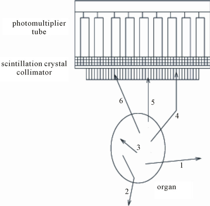
Figure 1. Detection of photons in the gamma camera.
data leads to improved reconstructions. A wide range of medical techniques, such as PET and SPECT, use appropriate algorithms to improve the reconstructions. Modelling of the physical factors like attenuation, scatter and absorption between the camera device and the organ of interest was studied by [20]. Experiments were designed to measure these factors and reconstruction performed from phantom and with real patient data. Extension of their process was the work of [24] who estimate the parameters of the proposed model using maximum likelihood.
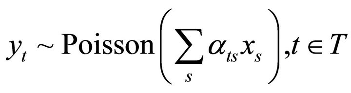
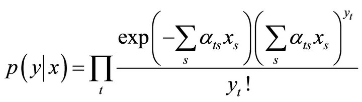
Let the true spatial distribution of radioisotope be denoted as x, and x(u) denote the isotope concentration at spatial location u Î R3. The data, which are an array of detected photons collected by the gamma camera, are described by the random variables , where t denotes a single detector tube. Since each photon is detected in at most one tube and emissions from u are assumed to be random, then the generally accepted model states that the pixel values in the recorded image, y, follow a Poisson distribution. The recorded counts are thus independent Poisson random variables with
  with
with  and
and  is the mean rate of arrivals at detector t from emissions from a point source of unit concentration at u. The weights
  express the physical factors of absorption and scattering inside the body and the geometrical factors which are defined by the detector system. This statistical model for the data is essentially that which applies to general emission applications [4] and especially for PET applications (see [5,9]). For computational purposes the body is divided into equal rectangular pixels with values denoted by
 , where xs is the true concentration of radiopharmaceutical at pixel s. The yt are a sample from a Poisson distribution with expected values
 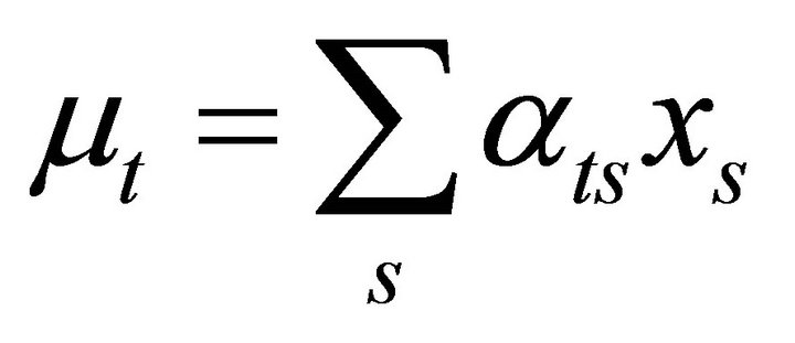 with
with  [5,912,25], which are given by
 (1)
(1)
where αts corresponds to the conditional probability that an emission at s is detected in tube t, and the sum is over the set of pixels which specify the body space. The {αts} are called weight coefficients and their modelling depends on the geometry of the gamma camera system, the physical shape of the body and the properties of the emitted photons. The important factors for modelling the weight, ignoring patient effects, are: 1) the proportion of radioactivity that has not decayed by the time at which data are collected, 2) the proportion of emissions that survive attenuation, 3) the angle of view from the centre of pixel s into detector t, or the solid angle when the third-dimension is considered. The most important of these are attenuation and angle of view, which have been studied by [20,23,24].
3. Bayesian Modelling
The use of maximum likelihood as a guiding principle in the process of reconstruction was studied by [4,8,25]. The requirements for the general model are:
• the data model (likelihood) p(yjx), and
• the prior model p(x).
The aim is to specify the posterior density  of x given the data y. Based on Bayes’ theorem the posterior density
  is given by
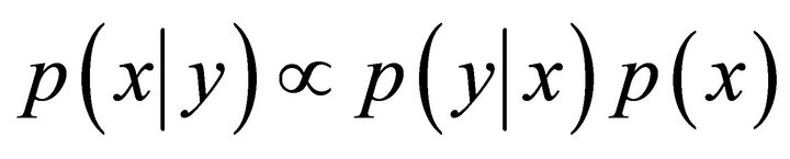 (2)
(2)
In SPECT the prior distribution models any available prior information which relates to the true isotope concentration. The concentration could be smooth for some areas but between others there may be sharp changes. This prior information introduces a penalty which leads to smoothness in the resulting reconstruction. The appropriate formula for the prior distribution is a pairwise difference, Gibbs prior, with a potential function that incorporates smoothing and scale parameters. [4,8,12,20,25] proposed a prior based on the Gibbs distribution with form:
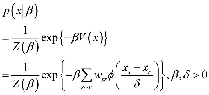 (3)
(3)
where  is the normalizing constant with
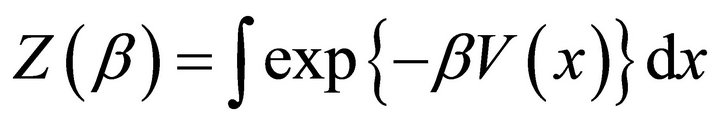 . In SPECT the concentration could be smooth for some areas but between others there may be sharp changes. This prior information introduces a penalty which leads to smoothness in the resulting reconstruction. In the above, V is called the energy function and
  the potential function; β is a smoothing parameter and δ a scale parameter; s ~ r indicates that pixel s is a neighbour of pixel r and wsr is a weighting factor. Note that the parameter β controls the degree of correlation between neighbouring pixels and hence the smoothness of the reconstruction. If
  then no spatial variation occurs and if
  then spatially unstructured variation appears. The form of {wsr} depends on the type of neighbourhood system, here a second order neighbourhood is used with
  if s and r are orthogonal nearest neighbours and
  if s and r are diagonal nearest neighbours. The form of the
  function defines a Markov random field with a particular neighbourhood structure (say first or second order). The function
  is non-negative, symmetric about zero and monotonically increasing for positive values and decreasing for negative values.
4. Estimation Algorithm
For SPECT applications, the joint probability function of the data given the isotope concentration is
 (4)
(4)
which leads to the log-likelihood
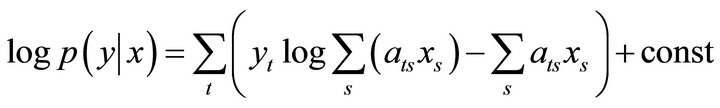 (5)
(5)
The aim is to maximises  with respect to x. The EM-algorithm is a general approach to iterative optimisation of likelihoods where the data can be formulated in an incomplete/complete specification. In SPECT, the data are described as incomplete whereas the complete data are needed to estimate the isotope concentration. The EM-procedure introduces the missing data zts which are defined as the number of photons that are emitted from pixel s and detected in detector t. The complete data includes the missing data zts and the incomplete data yt. Starting from a positive solution, the algorithm iterates until convergence, although the rate of converge is slow. Considering the unsatisfactory results of the maximum likelihood estimation, [3,13,21,23,25] shows that the noise in the reconstructions occurs when climbing the likelihood hill towards the maximum, a result which agrees with the experiments presented by [4,5]. An extension of their work was the iterative algorithm suggested by [2] which includes a penalty function controlling the smoothness of the reconstruction. The penalty function is related to the prior model and combined with the likelihood to form the penalised likelihood. The resulting estimation algorithm is a modification of the EM-algorithm, called the One Step Late or OSL-algorithm [2]. The inclusion of the prior distribution
  leads to maximum a posteriori estimation (MAP estimation). The aim is to maximise the log-posterior density
  with form
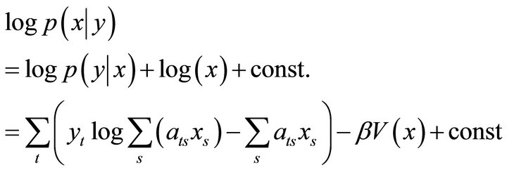 (6)
(6)
The OSL-approach is successful in overcoming the noise effects of the EM algorithm. The rate of convergences is slower. ML deteriorates, but MAP stays stable near the optimum solution.
5. Relationship between β Values and Distances
Figure 2 shows reconstructions using different β values for small and large distances. From the visual comparison it is clear that for small distances the reconstructions are closer to the truth as well as for small β values. Measure for comparison has been considered the Root Square Error (RSE) between reconstruct and truth, number of iterations for the convergences of the algorithm and CPU execution time.
The amount of smoothing in the reconstructions shown in Figures 2(b) and (c) is very similar. To achieve the level of smoothing in Figure 3(a) but using s = 40 cm would require a substantial reduction in β. Similarly a substantial increase in β would be needed to reproduce the smooth reconstruction showing in Figure 3(b) for s = 15 cm. This suggests that a relationship between β and s exists.
Summarising these results the conclusions are:
• When the camera is close to the body the reconstructions are better compared to the results when the camera distance is far from the body. The running times, the number of iterations and the RSE increase as the distance increases.
• When the β value is smaller, the RSE is decreased compared to large β values. The β value controls the smoothness of the reconstructed image, so small β values give better reconstruction.
• A relationship between β and camera distance exists.
The optimal β values will be found for different distances and a model fitted between β and distance. The optimal value of β is the value which minimises the RSE measure.
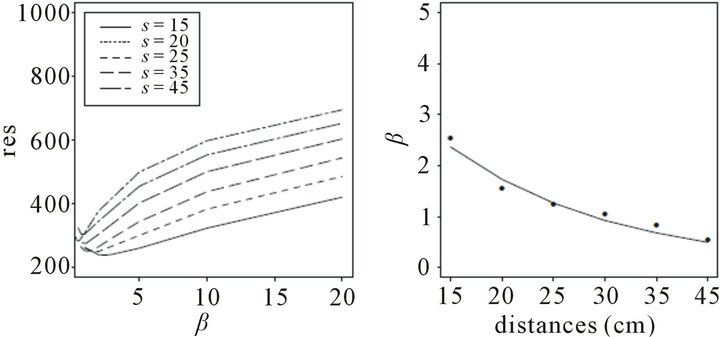
Figure 3(a) shows the RSE for different β values and different camera distances. For each value of s the RSE initially decreases as β increases, then rapidly increases. The optimal value, βopt, can be found as the minimum of RSE. The concentration of minimum values occurs when β is small. This result agrees with other authors (Green, 1990; Weir and Green, 1994) who have suggested that satisfactory reconstructions require small β. The optimal β values are presented in Figure 3(b) and Table 1, along with fitted values. As the distance increases the βopt value gets smaller. These results are based on data simulated using the approximate solid angle formula; results using the exact solid angle formula are identical.
After some experiments with models from different families, the best fit model between distance (s) and optimal β value is given by [23]:
 (7)
(7)
with  with an R2 value of 96%. The estimated values based on this model are given in Table 1. Comparing the optimal values and the estimated values it is clear that the estimated values are very close for all distances.
5.1. Circular Rotation
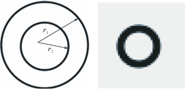
Experiments based on the elliptical rotation system will be presented using data from the artificial truth. For the artificial truth representation, two circles are considered which represent a solid inner cylinder placed centrally within a larger hollow cylinder. The radius of the inner circle is r2 = 8 cm and the radius of the outside circle is r1 = 12 cm (Figures 4(a) and (b)).
This “truth” is similar to the phantom used by [21,23] and represents a simplified 3d model of the left ventricular myocardium with homogeneous uptake of Tl-201.
For this rotation system, two distances are defined: the minor-axis radius (rx) and the major-axis radius (ry). Throughout ry is fixed at 40cm and results of the examination of the reconstructions for different distances, rx = 15, 25, 35 cm, are presented. In the following figures, rx
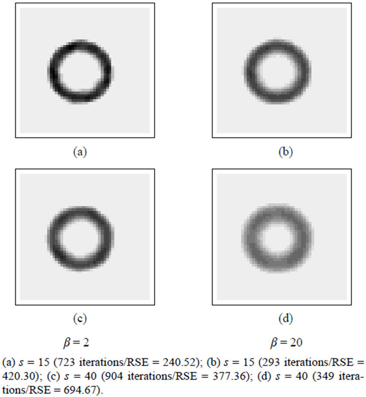
Figure 2. Reconstructions for different distances using β = 2 and β = 20.
 (a) (b)
Figure 3. Relationship between distances and βopt values.
 (a) (b)
Figure 4. (a) Description of artificial truth; (b) 2-dimensional representation.
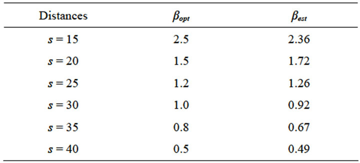
Table 1. Optimal and fitted β values.
is shown in the horizontal direction and ry in the vertical direction.
The reconstructions for the two β values (2 and 20) are displayed in Figure 5 and the resulting comparison measures for the different distances are given in Table 2. It is clear that as the distance rx increases the reconstructions become smoother. The smoothness has the effect of increasing the RSE, number of iterations and running time for both choices of β. For the small β value  and camera distance close to the body
 , the reconstruction is close to the truth with sharp boundaries. However, the amount of smoothing is larger in the areas where the camera is closest to the body (that is the sides of the ring). The algorithm needs 839 iterations to reach the final reconstruction, with RSE quite small (314.76). As the distance increases the boundaries become less sharp, and the differences in smoothing disappear.
For the larger β the reconstruction is smoother especially at the sides of the ring. This has the effect of increasing the RSE to 588.10, and decreasing the number of iterations to 312. The same pattern of results, as for β = 2, is obtained as rx increases. The resulting reconstructions lead to the same conclusion as in the circular rotation and hence a different choice of β is needed for different distances.
To investigate the relationship between distance and β, an optimal value for β could be found, as in the circular rotation. For the elliptical rotation the process to find the optimal value is harder because of the dimension of the
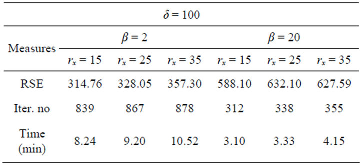
Table 2. Comparison of the measures for different distances using β = 2 and β = 20.
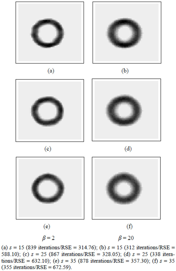
Figure 5. Reconstructions for different distances using β = 2 and β = 20.
problem. The optimisation for β could be done by minimising the RSE for all combinations of the two distances . A 3D graph would be needed with x-axis representing the vertical distance, y-axis the horizontal distance and z-axis the values of β that minimise the RSE. As can be imagined, this process needs a lot of computational time and would depend on the form of artificial truth. A reasonable approximation is to use the relationship from the circular rotation. The choice of β could be done using the relationship between only one distances rx or ry. For the first choice, rx, the related areas are correctly smoothed but those related to ry are over-smoothed. Conversely using ry, the related areas are correctly smoothed but the areas related to rx are under-smoothed. An appropriate choice of βopt is likely to be between the two β values. One approach is to use the β value corresponding to the average of the distances, alternatively the average of the two β values. These procedures mean that some areas are over-smoothed relative to an ideal β value and others are under-smoothed.
5.2. Elliptical Rotation
The elliptical rotation system is based on two distances, one which corresponds to the camera close to the body and the other to the camera far from the body. The effect of this is that the spatial resolution varies across the reconstruction. By visual comparison it was clear that in the regions where the camera was close to the body, the reconstruction was close to the truth with sharp boundaries. Alternatively, for the regions where the camera was far away, the reconstruction was smoother. This has the effect that uniform regions are reconstructed as nonuniform, which agrees with a remark of [21,23]. The method which is proposed in this section balances the distances in such a way that the resulting reconstruction will be closer to the truth.
The truth could be divided into four regions, where two regions correspond to the small distances and the other two to the large distances. Based on this, the image model was split into nine regions, as represented in Figure 6. Each region has a different β value which controls the amount of smoothing within the region. The areas where the camera is closest, A1, take the value of β corresponding to the distance rx and the areas where the camera is furthest away, A2, take the value of β corresponding the distance ry; the remain five regions take the average of the β values for A1 and A2. This method will uses inhomogeneous Markov random fields structure [6,7,10,26] and it is referred to as the block-β method.
The methods was applied to data obtained using distances  and
and , the resulting reconstruction is given in Figure 7 and summary measures in Table 3. The β values for region A1 is 2.5, for A2 is 0.5 and for the remaining regions 1.5. The reconstruction from
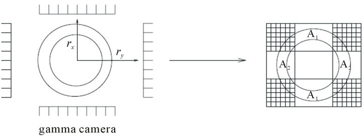
Figure 6. Classification of the regions for different β values.
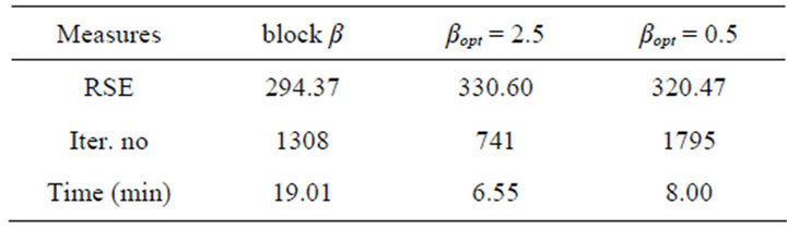
Table 3. Comparison of block-β method and single β.

Figure 7. Reconstructions for block-β method and for single β.
the block-β method is compared to the reconstructions using the optimal value for distances 15 cm  and 40 cm
 .
.
Comparison of the reconstructions shows that the block method performs better with RSE equal to 294.37 compared to 330.60 and 320.47. The algorithm needs 1308 iterations to reach the final reconstruction which is between the other two values, as expected. The running time is more than twice that of the other two, however this is likely to be due to the implementation of the algorithm.
6. Conclusions
This work studies the relationship between choice of β and camera distance. From experimental results using circular camera rotation, it was clear that a relationship between β value and distances exists. Optimal β values were found for different distances and a model was fitted to these values. The optimal β values were found by minimising the RSE.
The second part of the work looks at the elliptical camera rotation system, where major and minor axis distances are defined. From experiments the same relationship between β and distance was apparent. For single β the variation of distance effects the reconstructions, especially in the region where the camera is closest to and furthest from the body; the RSE measure is bigger and the algorithm needs more iterations to converge. An optimisation procedure could be used as for circular rotation, but due to excessive computational time, the method seemed inappropriate. Instead the relationship from the circular system was used to choose a β value using a single distance. Comparison of the RSE suggests that the reconstructions are reasonably close to the truth, but the shape of the ring is distorted. To counteract this distortion, the block β method was proposed. The main idea of the method is to balance the effects of the variation of the distances by changing the amount of smoothing. The image model was split into subregions based on distance to the camera. The subregions take the optimal β values which are given by the fitting model from the circular camera rotation system. As a result of this method, the shape of the ring appears closer to the truth.
REFERENCES
- S. A. Larsson, “Gamma Camera Emission Tomography,” Acta Radiologica, No. S363, pp. 1-75.
- P. J. Green, “On Use of the EM Algorithm for Penalized Likelihood Estimation,” Journal of the Royal Statistical Society, Series B, Vol. 52, 1990, pp. 443-452.
- B. Chalmond, “An Iterative Gibbsian Technique for Simultaneous Structure Estimation and Reconstruction of M-Ary Images,” Pattern Recognition, Vol. 22, No. 6, 1989, pp. 747-761. doi:10.1016/0031-3203(89)90011-3
- L. A. Shepp and Y. Vardi, “Maximum Likelihood Reconstruction in Positron Emission Tomography,” IEEE Transactions on Medical Imaging, Vol. 1, No. 2, 1982, pp. 113-122. doi:10.1109/TMI.1982.4307558
- Y. Vardi, L. A. Shepp and L. Kauffman, “A Statistical Model for Positron Emission Tomography,” Journal of the American Statistical Association, Vol. 80, No. 389, 1985, pp. 8-37. doi:10.1080/01621459.1985.10477119
- J. Besag, “Spatial Interaction and the Statistical Analysis of Lattice Systems,” Journal of the Royal Statistical Society, Series B, Vol. 36, 1974, pp. 192-236.
- J. Besag, “Discussion of Paper by P. Switzer,” Bulletin of the International Statistical Institute, Series A, Vol. 332, 1986, pp. 323-342.
- S. Geman and D. Geman, “Stochastic Relaxation, Gibbs Distribution and the Bayesian Restoration of Images,” IEEE Transactions on Pattern Analysis and Machine Intelligence, Vol. 6, No. 6, 1984, pp. 721-741. doi:10.1109/TPAMI.1984.4767596
- T. Hebert and R. Leahy, “A generalized EM Algorithm for 3D Bayesian Reconstruction from Poisson Data, Using Gibbs Priors,” IEEE Transactions on Medical Imaging, Vol. 8, No. 2, 1989, pp. 194-202. doi:10.1109/42.24868
- G. R. Cross and A. K. Jain, “Markov Random Field Texture Models,” IEEE Transactions on PAMI, Vol. 5, No. 1, 1983, pp. 25-39. doi:10.1109/TPAMI.1983.4767341
- R. G. Aykroyd, “Bayesian Estimation of Homogeneous and Inhomogeneous Gaussian Random Fields,” IEEE Transactions on PAMI, Vol. 20, No. 5, 1998, pp. 533-539. doi:10.1109/34.682182
- D. M. Higdon, J. E. Bowsher, V. E. Johnson, T. G. Turkington, D. R. Gilland and R. J. Jaszczak, “Fully Bayesian Estimation of Gibbs Hyperparameters for Emission Computed Tomography Data,” IEEE Transactions on Medical Imaging, Vol. 16, No. 5, 1997, pp. 516-526. doi:10.1109/42.640741
- I. S. Weir, “Fully Bayesian SPECT Reconstructions,” Journal of the American Statistical Association, Vol. 92, No. 437, 1997, pp. 49-60. doi:10.1080/01621459.1997.10473602
- M. K. Cowles and B. P. Carlin, “Markov Chain Monte Carlo Convergence Diagnostics: A Comparative Review,” Journal of the American Statistical Association, Vol. 91, No. 434, 1996, pp. 883-904. doi:10.1080/01621459.1996.10476956
- J. M. Hammrsley and D. C. Hanscomb, “Monte Carlo Methods,” Methuen, London, 1964. doi:10.1007/978-94-009-5819-7
- W. K. Hastings, “Monte Carlo Sampling Methods Using Markov Chains and Their Applications,” Biometrika, Vol. 57, No. 1, 1970, pp. 97-109. doi:10.1093/biomet/57.1.97
- A. D. Sokal, “Monte Carlo Methods in Statistical Mechanics: Foundations and New Algorithms,” Cours de Troisieme Cycle da la Physique en Suisse Romande, Lausanne, 1989.
- J. G. Propp and B. D. Wilson, “Exact Sampling with Coupled Markov Chains and Applications to Statistical Mechanics,” Random Structures and Algorithms, Vol. 9, No. 1-2, 1996, pp. 223-252. doi:10.1002/(SICI)1098-2418(199608/09)9:1/2<223::AID-RSA14>3.0.CO;2-O
- D. Geman and G. Reynolds, “Constrained Restoration and the Recovery of Discontinuities,” IEEE Transactions on PAMI, Vol. 14, No. 3, 1992, pp. 367-383.
- S. Geman and D. E. McClure, “Statistical Methods for Tomographic Image Reconstruction,” Bulletin of the International Statistical Institute, Vol. 52, No. 4, 1987, pp. 5-21.
- R. G. Aykroyd and S. Zimeras, “Inhomogeneous Prior Models for Image Reconstruction,” Journal of American Statistical Association, Vol. 94, No. 447, 1999, pp. 934- 946. doi:10.1080/01621459.1999.10474198
- D. Chandler, “Introduction to Modern Statistical Mechanics,” Oxford University Press, New York, 1978.
- S. Zimeras, “Statistical Models in Medical Image Analysis,” Ph.D. Thesis, Department of Statistics, Leeds University, 1997.
- I. S. Weir and P. J. Green, “Modeling Data from Single Photon Emission Computed Tomography,” Advances in Applied Statistics, Vol. 21, No. 1-2, 1994, pp. 313-338.
- J. Besag, P. J. Green, D. Higson and K. Mengersen, “Bayesian Computation and Stochastic Systems,” Statistical Science, Vol. 10, No. 1, 1995, pp. 3-41.
- J. Besag, “On the Statistical Analysis of Dirty Pictures,” Journal of the Royal Statistical Society, Series B, Vol. 48, No. 3, 1986, pp. 259-302.