Computational Water, Energy, and Environmental Engineering
Vol.06 No.03(2017), Article ID:78017,16 pages
10.4236/cweee.2017.63020
Modeling of Unsteady Flow through Junction in Rectangular Channels: Impact of Model Junction in the Downstream Channel Hydrograph
Seidou Kane1*, Soussou Sambou1, Issa Leye1, Raymond Diedhiou1, Seni Tamba2, Mouhamed Talla Cisse2, Didier Maria Ndione1, Mousse Landing Sane1
1Faculty of Sciences and Technics, Department of Physics, Cheikh Anta Diop University, Dakar, Senegal
2Polytechnic High School of Thies, Thies, Senegal

Copyright © 2017 by authors and Scientific Research Publishing Inc.
This work is licensed under the Creative Commons Attribution International License (CC BY 4.0).
http://creativecommons.org/licenses/by/4.0/


Received: May 7, 2017; Accepted: July 25, 2017; Published: July 28, 2017
ABSTRACT
Open channel junctions are encountered in urban water treatment plants, irrigation and drainage canals, and natural river systems. Junctions are very important in municipal sewerage systems and river engineering. Adequate theoretical description of flow through an open channel junction is difficult because numerous variables are to be considered. Equations of junction models are based on mass and momentum or mass and energy conservation. The objective of this study is to compare two junction models for subcritical flows. In channel branches, we solve numerically the Saint-Venant hyperbolic system by combining Preissmann scheme and double sweep method. We validate our results with HEC-RAS using Nash and Sutcliffe efficiency. In junction models, equality of water stage and complete energy conservation equation from HEC-RAS are compared. Outcome of the research clearly indicates that the complete conservation energy model is more suitable in flow through junction than equality of water stage model in serious situations.
Keywords:
Junction Model, HEC RAS, Saint-Venant’s Equations, Double Sweep Method, Equality of Water Stages, Energy Conservation, Modelling of Flow

1. Introduction
Channel junctions are area of separation or meeting of natural or artificial flow networks. They are often encountered in open channel networks of drainage systems and river systems [1] . The efficiency of free surface drainage systems such as drainage systems in urban areas depends highly on the correct functioning of the junction viewpoints: the failure of one single junction may threaten the functioning of the entire network [2] . Channel junctions are one of the most crucial hydraulic structures in natural and artificial free surface flows. Flow at junction is characterized by tri-dimensional effects and presence of an air-water mixture. It includes also complicated patterns with a separation zone immediately downstream, low pressure, low turbulence intensities and complex velocity distributions [3] . These characteristics make mathematical solutions considerably complicated. An adequate theoretical description of flow through junction requires external and interior boundary conditions. External boundary conditions for the junction are calculated by solving numerically the Saint-Ve- nant’s equations (1871). Interior boundary conditions are a set of compatibility relationships based on the mass and energy conservation or on mass and momentum conservation. Mass and momentum conservation based models allow more realistic representations by taking into account the angle of inclination of the junction [4] [5] [6] . This kind of model uses a set of nonlinear equations and Vasquez et al. [7] showed that in serious situations, these models are more suitable. Wu et al. [1] studied open channel junction flow with a depth averaged numerical model for open channel flows without the rigid-lit assumption, but with consideration of the important effect due to the bottom and the surface. Sivukamar [8] presented a 3D numerical simulation of horizontal bed open channel water flow with 90˚ equal width junction. The numerical solution of these equations takes into account all physical aspects of flow through the junction, but they are very complicated and difficult to implement [9] . Mass and energy based models are more easy to implement, avoid solving non linear equations, and provide answer in much less time than solution procedures based on momentum models. It can be simplified when physical effects such as boundary effects can be neglected, or when the flow through the junction is subcritical. This model may then simply be reduced to the equality of water surface elevations model also referred as stages equality model [10] [11] . Water surface elevations based model are very popular among the hydraulic engineers for all above mentioned reasons. Several applications like Mike 11, Mouse Model from the Danish Hydraulic Institute (1999), Canoe model from SOGREAH and Insavalor (2009) and InfoWorks from Wallingford Software (2006) use the water stage equality at the junction [11] . Other applications such as HEC RAS use directly mass and energy based model. HEC RAS is integrated free software designed by the Hydrologic Engineering Center of the U.S Army Corps of Engineers for hydraulic analysis which allows simulating free-surface flows. HEC RAS is a new version of the hydraulic model previously named HEC-2 that now includes a graphical interface for editing, modifying, and visualizing input data, as well as observing the results obtained. It is easy to navigate even for users with minimal modeling experience and can run quickly for real-time forecasting [12] . It is currently used in several engineering firms and government agencies [13] [14] [15] and it performs well flow through junction.
The objective of the present work is to show that the energy based junction model is generally more suitable than the equality of water stage junction model and should be applied in serious situations. We so compare the equality of water stage model, to the mass and energy model for a junction system. We calculate the external boundaries of the junction by solving Saint Venant’s equations using Preissmann scheme for discretization and double sweep method for numerical solution along the channels of the network. Our calculations are validated by HEC-RAS software. Inputs of the network are simple and complex hydrographs. We then apply equality of water stage model to the junction. We then use HEC-RAS mass and energy based junction model for the same network with the same conditions. The two junction models are compared at the output of the network.
2. Materials and Methods
A junction system is composed by three channels at least: two upstream channels and a downstream channel (Figure 1). Flow in the channels is simulated by solving numerically Saint-Venant’s equations. Two models can be used for interior boundaries of the junction: mass and energy conservation method or mass and momentum conservation method. The first can be simplified to the equality of water stage model.
2.1. Numerical Solutions in Branches Using Double Sweep Method
The one-dimensional Saint-Venant equations are used to model transient open- channel flow for an incompressible homogeneous fluid. Saint-Venant model is a nonlinear hyperbolic system of two equations based on mass conservation and momentum conservation laws. The first (1a) is the continuity equation, and the second (1b) is the momentum equation.
 (1)
(1)
where Q = discharge; A = cross-sectional; g = acceleration due to gravity; Z =

Figure 1. Junction’s characteristics.
elevation of the water surface, Sf = energy slope; t = temporal coordinate and x = longitudinal coordinate. Complete Saint-Venant’s system is very popular among hydraulic engineers and hydrologists but have no analytical solutions so numerical solutions have been developed. Many numerical methods have been proposed for discretization: implicit or explicit [16] . Implicit scheme is very interesting because it is not subject to the Courant-Friedrichs-Levy stability condition [17] . Among implicit schemes, the Preissmann one is the earliest used by hydraulicians. It is a compact method using only four grid points for the solution and thus minimizes the damage done by the interpolated function. It was used in real situation and programmed with the details necessary to provide answers to real problems [18] . The generalized Preissmann scheme is presented in Figure 2.
For a given space and time function , Preissmann scheme’s discretization is expressed as :
 (2)
(2)
 (3)
(3)
 (4)
(4)
where j is the space index, n the time index and ,
,  are weighting coefficients. The Preissmann scheme is second-order accurate in both time and space if
  and
and , and first-order accurate otherwise. Linear stability analysis shows that the centered scheme (
 ) is unconditionally stable for
  [18] .
Introducing Equations (2), (3) and (4) in Equations (1a) and (1b), we obtain two nonlinear algebraic equations:

Figure 2. Preissmann scheme.
 (5)
(5)
 (6)
(6)
The system is then linearized around an equilibrium steady-state by Taylor series expansion using Equations (7), (8) and (9):
 (7)
(7)
 (8)
(8)
 (9)
(9)
The following finite difference linear system is finally obtained:
 (10)
(10)
where ,
,  ,
,  ,
,  ,
,  ,
,  ,
,  ,
,  ,
,  and
and  are coefficients resulting from the linearization. Equations (10a) and (10b) must be solved for all computational points for every time step during the period of computation and any standard resolution method can be applied if the boundary conditions are also linearized. They are written for every reach connecting two nodes on the computational domain. Thus for a domain of N computational points there are 2N-2 discretized equations. Since there are two unknowns at each node, there are 2N unknowns in the domain, so two boundary conditions are needed to close the system [19] .
In this paper, we use the double sweep method as applied by Preissmann and Cunge. The number of elementary operations necessary to solve the system by this method is proportional to the number of points N while standard methods of matrix inversion is proportional to . A short presentation is described below:
The rating curve  is generally non linear. But locally, around a spatial point
 ,
,  and
and  can be considered enough small to assume there a linear relationship of the type of Equation (11) [18] [20] :
 (11)
(11)
We eliminate  in the Equations (10a) and (10b) by multiplying the first equation by
 , the second by
  and we obtain the Equation (12):
 (12)
(12)
Equation (12) is written again as follows:
 (13)
(13)
where:
 (14)
(14)
 (15)
(15)
 (16)
(16)
Substitution of Equation (11) into Equation (10a) leads to:
 (17)
(17)
Then replacing  in Equation (17) by its value in (13), we obtain Equation (18):
 (18)
(18)
Rearranging Equation (18) finally leads to:
 (19)
(19)
where:
 (20)
(20)
 (21)
(21)
Equation (19) represents the recurrence relation at point . The coefficients
  and
and  can be known for any point
  if the analogous coefficients
  and
and  are known at the previous point j.
We start the calculations from the upstream by setting the hydrograph Q(t) for . According to Equation (11), coefficient
  should be equal to zero because
  is independent of
 , so:
, so:
 and
and 
At the downstream boundary ( ),
), should be known. We retained a uniform flow rating curve. In this case using Manning-Strickler’s law we can compute
  and
and  by:
by:
 (22)
(22)
 (23)
(23)
2.2. Numerical Solutions in Branches Using Hec-Ras Software
To validate our results, we need to compare them with a known package. Many packages can solve unsteady flow with Saint-Venant’s equations with appropriate formulation to take into account the complexity of free surface flow. The HEC-RAS software solves the one dimensional unsteady flow equations by writing Saint-Venant equations in a general formulation for 1D flow in flood plain as follow [21] :
 (24)
(24)
 (25)
(25)
Subscripts (c) is associated to channel and (f) to floodplain,  is the total flow,
  is a coefficient,
  is the conveyance.
In our application the channels are rectangular and there is no flow over the banks. Thus the system of equations used by Hec-Ras becomes the same as the system of Equations (1a), (1b) described previously.
Numerical solution program of Saint-Venant used in HEC-RAS is based on the U.S. Army Corp of Engineer’s (USACE) model Unsteady Network Model. This program solves the mass conservation and momentum conservation equations with an implicit linearized system of equations using Preissman’s second order box scheme. The simultaneous system of equations generated for each time step (and iterations within a time step) are stored with a skyline matrix scheme and reduced with a direct solver developed specifically for unsteady river hydraulics by Dr. Robert Barkau. The state variables for the numerical scheme are flow and stage, which are computed and stored at each cross section. The hydraulic resistance is based on the friction slope from the empirical Manning’s equation, with several ways of modifying the roughness. Roughness can be characterized with Manning’s (n) or roughness height’s (k) (William E. F. 2003).
2.3. Junction Models
Numerical models junction in open channel networks are based on the mass conservation associated either to the energy conservation or to the momentum conservation [4] [7] .
2.3.1. Hec-Ras Junction Model
Stream junctions can be modeled by two methods within Hec-Ras: energy conservation or momentum conservation. The energy based method (EBM) has been used here. The main assumptions of this method are [4] [18] : resistance terms and lateral pressures are neglected; streamline curvature is considered small and vertical acceleration negligible so that the vertical pressure distribution is assumed to be hydrostatic; at the inflow and outflow sections, velocity distribution is uniform; the influence of the lateral flow angle is insignificant. This method solves the water surfaces across the junction by performing standard step calculations through the junction with the one dimensional energy equation. It does not take into account the angle of any of the tributary flows. The general equation between two sections is given below.
 (26)
(26)
where:  = elevation of the main channel invert at cross section j;
 = depth of water at cross section j;
 = average velocity cross section j;
  = energy head loss;
 = velocity weighting coefficient at cross section j.
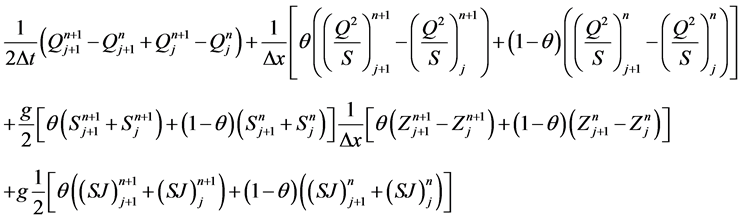
Subcritical flow calculations are performed up to the most upstream section of branch 3. The water surface at branch 1 is calculated by performing a balance of energy from station 3.0 to station 4.0. Friction losses are based on the length from station 4.0 to 3.0 and the average friction slope between the two sections (Figure 3). Contraction and expansion losses are also evaluated across the junction. The energy equation from station 3.0 to 4.0 is written as follows [21] :
 (27)
(27)
The water surface for the downstream end of branch 2 is calculated in the same manner.
2.3.2. Equality of Water Surface Model
Energy losses and differences in velocity head are difficult to evaluate, so that the interior boundary conditions may simply diminish to the equality of water surface elevations (Equation (28)) associated to the macroscopic version of continuity equation (Equation (29)), as in many software such as the One Dimensional Hydrodynamic Model Environment Canada 1988; Mike 11 model Danish Hydraulic Institute 1999; and Chaudhry 1993. The equations of the model are written as follows:
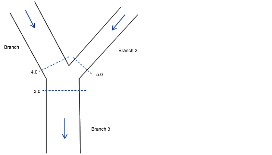
Figure 3. Junction model application by HEC RAS.
 (28)
(28)
 (29)
(29)
3. Applications and Results
3.1. Characteristics of the Hydraulic System
The network is represented by three identical rectangular branches related by a junction (Figure 4).
The geometric and hydraulic characteristics of the system are given in Table 1 (length, width, slope, and roughness). The numerical parameters (space step, time step, weighting coefficient) used in the double sweep method and in Hec- Ras software are presented in Table 2.
・ Upstream boundary conditions
At the input of the upstream branches constituting the junction, we chose a simple Henderson sinusoidal hydrograph (HS, Equation (30)), a two complex Henderson hydrographs, one with two equal peaks (HC2, Equation (31)), and another with three decreasing peaks (HC3D, Equation (32)). The corresponding hydrographs are shown in Figures 5-7.
 (30)
(30)
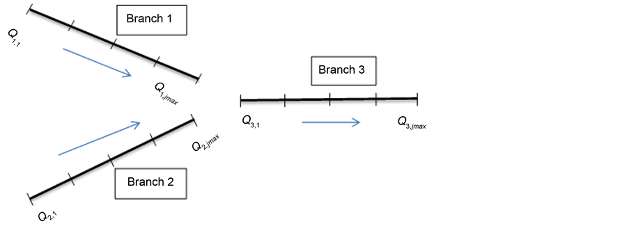
Figure 4. Hydraulic system.

Table 1. Characteristics of the network system.
Table 2. Numerical parameters.

Figure 5. Simple henderson hydrograph (HS).

Figure 6. Complex henderson hydrograph (HC2).
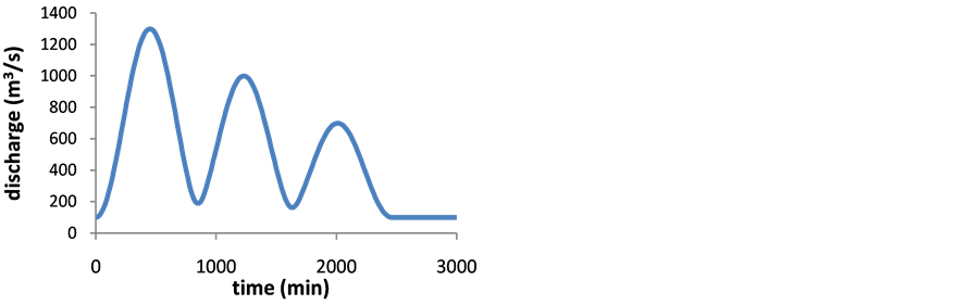
Figure 7. Complex henderson hydrograph (HC3D).
with


 (31)
(31)


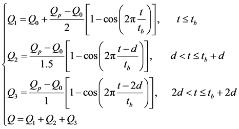 (32)
(32)


・ Downstream boundary conditions.
For downstream boundary conditions we have chosen a steady-state calibration curve:
 (33)
(33)
 = Manning’s coefficient;
  = hydraulic radius;
  = slope of the channel.
・ Initial condition is set by using a uniform flow with 
3.2. Criteria for Comparison
Hydrographs calculated according to our program are compared to those given by HEC RAS package. Two kind criteria are used for comparison: local criteria (Relative Peak Error or RPE, Equation (34); Relative Volume Error or RVE, Equation (35)) and global statistical criteria (Nash-Sutcliffe coefficient, Equation (36)).
 (34)
(34)
 (35)
(35)
 (36)
(36)
where  is the maximum discharge calculated by Hec-Ras;
  is the maximum discharge calculated with our program;
  is the volume by Hec- Ras;
  is the volume by our program;
  is discharge at time t,
  , are respectively and the mean of discharges calculated by Hec-Ras.
  is the discharge at time t calculated with our program (double sweep). Positive values of RPE and RVE correspond to under estimation and negative values to overestimation by our program. When these values are very small, the two methods of computation are equal. A NASH criterion close to 1 means a good representation of the hydrograph calculated by our program compared to that computed with HEC RAS.
4. Results and Discussions
There are two main characteristics of flow motion in channels: translation and attenuation. In translation, shape of the hydrograph is maintained along the channel while attenuation involves the reduction of the peak flow and the change of the shape of the hydrograph. Translation is dominant in steep straight channel, and attenuation is channel with storage. The downstream hydrographs are compared here.
We first validate our program in a single branch and then introduce the junction model.
・ Flow in a single branch (B1): model validation
We first compared downstream hydrographs of branch 1 that we have calculated to that computed with HEC-RAS. Corresponding results are presented in Figure 8. Criteria are presented in Table 3.
According to Table 3, RPE and RVE are very small, while Nash criterion is

Figure 8. Results at the downstream end of branch 1.
close to unity. This shows that our program reproduces well the flow in the channel compared to Hec-Ras model for simple and complex upstream hydrographs (Figure 8). It also lightly underestimates the peak flow while the volume of flow is almost the same. When we have a complex upstream hydrograph (Figure 6 and Figure 7) we obtain a simple hydrograph at the downstream end of the hydraulic system (Figure 8(b) and Figure 8(c)), this is due to the length of the branch. The channels of the system are very long so diffusion and also attenuation have to be more important and that makes the other peaks disappear.
・ Flow through the whole network with Junction models
We have then compared the hydrographs downstream the junction computed with the water surface equality method (EWS) to that of Hec-Ras junction method (EBM). Figure 9 shows the resulting hydrographs, and Table 4 the local and global characteristics.
Figure 9 shows a net difference between the hydrographs downstream of the
Table 3. Local and global characteristics in single branch B1.

Figure 9. Results at the downstream end of branch 3 after the junction.
Table 4. Local and global characteristics after the junction (branch 3).
junction obtained with the equality of the water surface (EWS) and that obtained by the energy based model (EBM): EWS junction model overestimates the peak flow and decreases the falling limb’s times of hydrographs when compared to EBM based model. We can see in Table 4 that RPE is negative and significant, the volume is slightly the same for the two approaches, and Nash criterion is relatively small but not very close to unity.
According to Figure 9, translation effect is more important in EWS model, while natural attenuation of hydrograph downstream the junction is well reproduced with EBM (HEC RAS). A theoretical justification of this fact is undertaken by comparing Equation (26) for EBM and (28) for EWS: it appears that the main difference in the pattern of hydrographs downstream of the junction between EWS and EBM model is due to the kinetic and friction losses terms at the junction. These terms are precisely those that lead to the attenuation of natural hydrograph observed during the propagation of the flood wave. It is obvious that neglecting these two terms impacts the shape of the hydrograph downstream the junction. This shows that EWS model is less suitable than EBM for junction. Simplified methods generally don’t have the accuracy of a solution procedure based on the complete equation. They can give sufficiently accurate results when all the assumptions are well defined and respected.
5. Conclusion
Junction in river network is represented by two kinds of model: mass and energy conservation and mass and momentum. Mass and energy conservation based models are easier to implement because they avoid solving numerically nonlinear equations. When flow is subcritical, mass and energy conservation model can be approximated by equality of water surface model as used in many packages. In this paper, we compared the equality of water surface (EWS) and the energy based model (EBM) for junction model. We solved numerically Saint- Venant equations using the four points PREISSMANN implicit scheme for discretization and the double sweep method in the channels of the junction and validated successfully the results with HEC RAS in the same conditions. Then we compared two mass and energy conservation based junction models: the equality of water surface based model (EWS) and the energy based model (EBM) use in HEC RAS software. Comparison of the patterns of the hydrographs downstream of the junction shows that EBM reproduces better dispersion and diffusion encountered in the natural flood wave propagation in river or channels. Analyzing the equations governing the two junction models, it appears that this can be due to the fact that EWS based model neglects kinetic energy and friction losses. In conclusion, although much easier to implement, the junction model based on the equality of water surface is less suitable in channel network.
Cite this paper
Kane, S., Sambou, S., Leye, I., Diedhiou, R., Tamba, S., Cisse, M.T., Ndione, D.M. and Sane, M.L. (2017) Modeling of Unsteady Flow through Junction in Rectangular Channels: Impact of Model Junction in the Downstream Channel Hydrograph. Computational Water, Energy, and Environmental Engineering, 6, 304-319. https://doi.org/10.4236/cweee.2017.63020
References
- 1. Wu, R. and Mao, Z.Y. (2003) Numerical Simulation of Open Channel Flow in 90-Degree Combining Junction. Tsighua Science and Technology, 8, 713-718.
- 2. Pfister, M., Gokkok, T. and Gisonni, C. (2013) Les jonctions avec les écoulements torrentiels. Séminaire VSA/EPFL Hydraulique des canalisations, Lausanne.
- 3. Baghlani, A. and Talebbeydokhti, N. (2013) Hydrodynamics of Right-Angled Channel Confluences by a 2D Numerical Model. IJST, Transactions of Civil Engineering, 37, 271-283.
- 4. Shabayek, S., Stiffler, P. and Hicks, F. (2002) Dynamic Model for Subcritical Combining Flows in Channel Junctions. Journal of Hydraulic Engineering, 128, 821-828. https://doi.org/10.1061/(ASCE)0733-9429(2002)128:9(821)
- 5. Hsu, C.C., Lee, W.J. and Chang, C.H. (1998) Subcritical Open Channel Junction Flow. Journal of Hydraulic Engineering, 124, 847-855. https://doi.org/10.1061/(ASCE)0733-9429(1998)124:8(847)
- 6. Bowers, C.E. (1950) Hydraulic Model Studies for Whiting Field Naval Air Station. Part V. Studies of Open-Channel Junctions. Saint Anthony Falls Hydraulic Laboratory Project Report No. 24.
- 7. Vasquez, J., Ghenaim, A., Ghostine, R., Kesserwani, G. and Mose, R. (2007) Simulation of Subcritical Flow at a Combining Junction. NOVATECH, 497-504.
- 8. Sivakumar, M., Dissanayake, K. and Godbole, A. (2004) Numerical Modeling of Flow at an Open-Channel Confluence. In: Mowlei, M., Rose, A. and Lamborn, J., Eds., Environmental Sustainability through Multidisciplinary Integration, Environmental Engineering Research Event, Australia, 97-106.
- 9. Brito, M., Canelas, O.B., Leal, J.L. and Cardoso, A.H. (2014) 3D Numerical Simulation of Flow at a 70° Open-Channel Confluence. V Conferência Nacional de Mecanica dos Fluidos, Termodinamica e Energia MEFTE 2014, Porto, Portugal APMTAC, 11-12 Setembro 2014.
- 10. Longxi, H. (2008). Parameter Estimation in Channel Network Flow Simulation. Water Science and Engineering, 1, 10-17. https://doi.org/10.1016/S1674-2370(15)30014-4
- 11. Ewemoje, T.A. and Abimbola, O.P. (2014) Verification of Coefficient of Rectangular Side Weirs Using Shabayek Model. Research Journal of Applied Sciences, 9, 397-401.
- 12. Sharkey, J.K. (2014) Investigating Instabilities with HEC-RAS. Unsteady Flow Modeling for Regulated Rivers at Low Flow Stages. Master Thesis, University of Tennessee, Knoxville.
- 13. Chandresh, G.P. and Gundaliya, P.J. (2016) Floodplain Delineation Using HECRAS Model—A Case Study of Surat City. Open Journal of Modern Hydrology, 6, 34-42. https://doi.org/10.4236/ojmh.2016.61004
- 14. Direction Departementale de L’equipement et de L’agriculture (DDE 42) (2010) Etude hydraulique de la rivière le gier et de ses affluents. Rapport d’étude hydraulique. Sogreah JCC/JMI 1741145 R2 MAI.
- 15. Smival (2011) Etude hydraulique de la Lèze: Simulation des crues synthétiques.
- 16. Fread, D.L. and Jin, M. (1997) Dynamic Flood Routing with Explicit and Implicit Numerical Solution Schemes. Journal of Hydraulic Engineering, 123, 166-173. https://doi.org/10.1061/(ASCE)0733-9429(1997)123:3(166)
- 17. Litrico, X., Pomet, J.B. and Guinot, V. (2010) Simplified Nonlinear Modeling of River Flow Routing. Advances in Water Resources, 33, 1015-1023.
- 18. Cunge, J.A. and Liggett, J.A. (1975) Unsteady Flow in Open Channels. Water Resources Publications. In: Mahmood, K. and Yevjevich, V., Eds., Chapter 4, Numerical Methods of Unsteady Flow Equations, Colorado, 89-182.
- 19. Meselhe, E.A. and Holly, F.M. (1997) Invalidity of Preissmann Scheme for Transcritical Flow. Journal of Hydraulic Engineering, 123. https://doi.org/10.1061/(ASCE)0733-9429(1997)123:7(652)
- 20. Preissmann, A. (1961) Propagation des intumescences dans les canaux et rivières. First Congress of the French Association for Computation, Grenoble, 433-442.
- 21. US Army Corp of Engineers Institute for Water Resources (2010) HEC-RAS River Analysis System Hydraulic Reference Manual Version 4.1. Davis.