Open Journal of Air Pollution
Vol.1 No.2(2012), Article ID:22751,8 pages DOI:10.4236/ojap.2012.12007
Micro-Scale Dispersion of Air Pollutants over an Urban Setup in a Coastal Region
1Center for Oceans, Rivers, Atmosphere and Land Sciences, Indian Institute of Technology Kharagpur, Kharagpur, India
2Fluidyn Software and Consultancy (P) Ltd., Bangalore, India
Email: *anvsatya@coral.iitkgp.ernet.in
Received July 19, 2012; revised August 25, 2012; accepted September 20, 2012
Keywords: CFD; PBL; Meso-Scale; Micro-Scale Dispersion
ABSTRACT
The dispersion of air pollutants is mainly governed by wind field and depends on the Planetary Boundary Layer (PBL) dynamics. Accurate representation of the meteorological weather fields would improve the dispersion assessments. In urban areas representation of wind around the obstacles is not possible for the pollution dispersion studies using Gaussian based modeling studies. It is widely accepted that computational fluid dynamics (CFD) tools would provide reasonably good solution to produce the wind fields around the complex structures and other land scale elements. By keeping in view of the requirement for the micro-scale dispersion, a commercial CFD model PANACHE with PANEPR developed by Fluidyn is implemented to study the micro-scale dispersion of air pollution over an urban setup at Indira Gandhi Centre for Atomic Research (IGCAR), Kalpakkam a coastal station in the east coast of India under stable atmospheric conditions. Meso-scale module of the PANACHE model is integrated with the data generated at the site by IGCAR under RRE (Round Robin Exercise) program to develop the flow fields. Using this flow fields, CFD model is integrated to study the micro-scale dispersion. Various pollution dispersion scenarios are developed using hypothetical emission inventory during stably stratified conditions to understand the micro-scale dispersion over different locations of coastal urban set up in the IGCAR region of Kalpakkam.
1. Introduction
The study of air pollution dispersion is pre-requisite for urbanization, industrial growth and expansion of coastal population [1,2]. The air pollution dispersion studies at various scales gives the information about local and long range scenarios impact [3]. Pollutants are generally generated in urban areas (mostly from vehicular traffic) and in industrial regions. Once they are generated, they get transported in the atmosphere by movement of air. In general, their movement is governed by a host of factors including meteorological conditions, topography of the local region and the nature of the pollutants themselves. The pollutants, while getting dispersed rarely move above the troposphere, which is the lowest level of the Earth’s atmosphere. The lowest part of the troposphere is known as the planetary boundary layer (PBL); this region is directly influenced by the earth’s surface in the form of frictional drag (from topology and obstacles like buildings etc.), solar heating (radiation) and evapotranspiration [4,5]. The PBL may extend up to 100 m to 3000 m from the ground. Dispersion in the micro-scale range almost always takes place wholly in the PBL. Atmospheric dispersion modeling is the mathematical summation of how air pollutions disperse in the ambient atmosphere. Some of the most important parameters that play a leading role in the dispersion of pollutants in the atmosphere are wind velocity, atmospheric turbulence, stability, temperature, humidity [6]. The pollutants get transported along the direction of wind, but it is the atmospheric turbulence that determines the lateral and vertical spread of the pollutants. Stability assumes a critical role in determining the amount of turbulence in the atmosphere and thus directly affects the level of dispersion. Most air pollution sources are located within the urban canopy layer and transport phenomenon are dominated by a number of complex factors like emission source characteristics, the turbulent structure of the wind as well as the local arrangement of building and structures [7]. In order to predict turbulent transport phenomena in built-up areas, a complex obstacle resolving type of dispersion model is required [8]. The flow around the obstacles such as buildings, trees and other natural roughness elements influence the dispersion of pollutants in the micro-scale. A plethora models are in development stage because the existing models are not capable to represent the flow around the obstacles. Hence, the utility of CFD (Computational Fluid Dynamics) based models are a good alternative to represent these complex flows. CFD models provide complex analysis of fluid flow based on conservation of mass and momentum by resolving the Navier-Stokes equation using finite difference and finite volume methods in three dimensions [9,10]. Various authors implemented variety of CFD models to study pollutant dispersion and deposition, wind-driven rain, building ventilation, etc. [11-15].
Turbulence is classically calculated using k - ε losure methods to calculate the isotropic eddy viscosity parameter present in both the momentum and pollution transport equations, which assumes that a pollutant is diluted equally in all directions [16]. This treatment performs well on a flat boundary layer [17]. However, when a stratified boundary layer exists the closure method needs to be modified to include the Coriolis force and reduced wind shear in the upper atmosphere. As a result an overestimation of the eddy viscosity is reported that lead different CFD models showed good agreement in overall wind flow field but demonstrated large differences in velocities and turbulence. In the present study, a commercial CFD model PANACHE with PANEPR developed by Fluidyn is implemented to study the micro-scale dispersion of air pollution over an urban setup in a coastal station in the east coast of India, i.e. Indira Gandhi Centre for Atomic Research (IGCAR), Kalpakkam. Understanding of atmospheric dispersion during nighttime is of paramount importance. During daytime, excessive heating and wind conditions result in good mixing, where as nighttime due to strong stable conditions, the mixing is reduced and has a different signature of dispersion of pollutants; some times it may leads to the occurrence of catastrophic episodes. Due to this important reason, in the present study, the nighttime to early morning hours are considered to see the dispersion scenarios.
2. Study Region
A meso-domain is chosen in the geographical coordinates of 12.2818˚N to 13.3200˚N and 79.5043˚E to 80.6603˚E. The size of the domain is 145 km × 110 km × 0.1 km. The meso-scale study domain is depicted in Figure 1. A micro-domain lies in the geographical coordinates of 12.5370˚N to 12.5770˚N and 80.1549˚E to 80.1950˚E. The micro-scale study domain is depicted in Figure 2. The study area is east coast of Tamilnadu includes the region of IGCAR, Kalpakkam. For this study, two domains were chosen: One is meso-domain and the other is micro-scale domain. The period of the study is 15 to 22 September 2010. There are 5 meteorological towers and 5 Automatic weather stations providing continuous measurements of wind speed, wind direction, air temperature, humidity and other variables related to turbulence and soil measurements. These meteorological data is available at 2, 8, 16, 32, and 50 m elevations from ground. In this study, wind speed, wind direction and air temperature at different heights are utilized. Geographical coordinates in terms of longitude and latitude of all specific locations in the study area are identified from satellite map provided by IGCAR, Kalpakkam are provided to the model for to develop terrain fields.
3. CFD Modeling Tool
Two CFD models namely PANACHE and PANEPR have been employed in the present study [18]. FluidynPANACHE is a computer code for numerical simulation of atmospheric flows and pollution, and uses CFD tools in a finite volume based approach to solve the differential
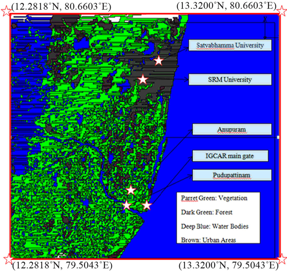
Figure 1. Mesoscale domain.
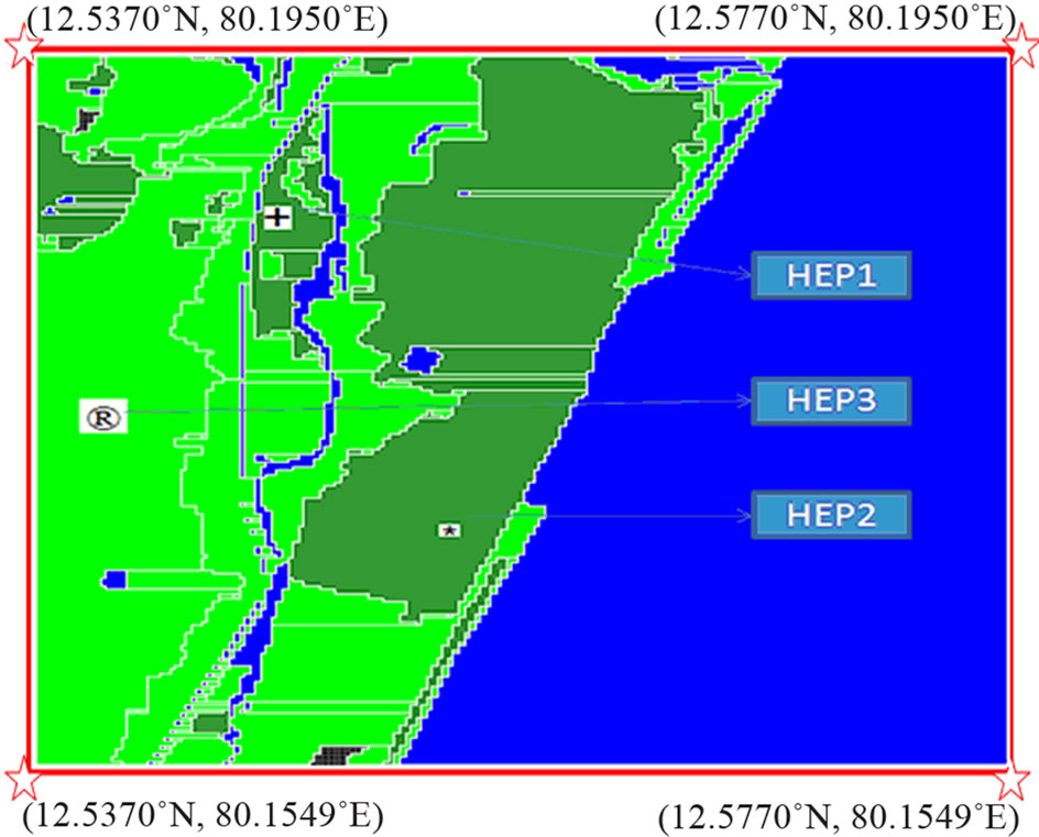
Figure 2. Micro-scale domain.
equations governing mass, momentum, and energy transfer (http://www.fluidyn.com/fluidyn/). It solves the mass, momentum, and energy conservation equations for both laminar and turbulent flow [19-22]. The equations for the two cases differ primarily in the form and magnitude of the transport coefficients (diffusivity, viscosity, and thermal conductivity). Eddy hypothesis is used to compute the turbulent contribution to the exchange coefficients.
The continuity equation for species m is
 (1)
(1)
 ;
;
ρm = mass density of species m;
ρ = total mass density;
u = fluid velocity;
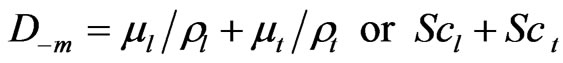
Dm = diffusion coefficient for species m in air;
ym = mass fraction of species;
m = ρm/ρ;
ρms = source term for species m due to pollutant emissions;
ρmd = source term for species m due to dry deposition in canopies;
ρmp = source term for species m due to droplet evaporation/condensation;
ρmc = source term for species m due to chemical reactions;
Scl = Schmidt number for laminar flow;
Sct = Schmidt number for turbulent flow;
µl = molecular viscosity of air;
µt = turbulent eddy viscosity.
We get the continuity equation for total fluid density
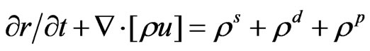 (2)
(2)
ρs = total mass source due to pollutant emission;
ρd = total mass source due to dry deposition in canopies;
ρp = total mass source due to droplet Evaporation and condensation.
The momentum equation for the fluid mixture is
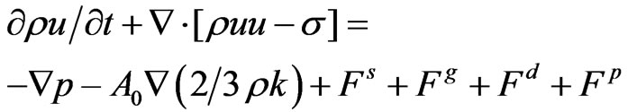 (3)
(3)
P = Pressure;
σ = Newtonian viscous stress tensor
=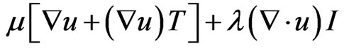 (4)
(4)
μ, λ = First and second coefficients of viscosity;
λ = −2/3μ;
T = transpose;
I = unit dyadic;
A0 = 1 when the k - e or the k - L turbulence model is active, = 0 otherwise;
k = turbulence kinetic energy;
Fs = rate of momentum gain per unit volume due to Pollutant emissions;
Fg = force due gravitational acceleration;
Fd = force due to plant canopy effect, dry deposition, etc;
Fp = force due to interaction with droplets/particles.
The internal energy equation is
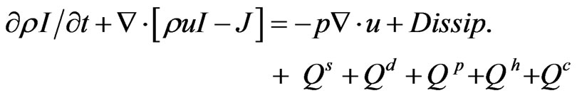 (5)
(5)
I = specific internal energy;
J = heat flux vector
=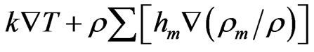 (6)
(6)
k = thermal conductivity;
T = Temperature;
hm = specific enthalpy of species m;
Qs = rate of specific internal energy gain due to pollutant emissions;
Qd = rate of specific internal energy gain due to dry depositions in canopies;
Qp = rate of specific internal energy gain due to interaction with particles;
Qh = rate of specific internal energy gain from surface energy budget;
Qc = rate of specific internal energy gain due to chemical reactions;
Dissipation = σ.![]() u for laminar flow
u for laminar flow
= ρε for turbulent flow.
4. Results and Discussion
4.1. Generation of Micro-Scale Domain Wind Field
In the study domain, several in situ meteorological measurement stations, i.e. masts and micro-meteorological towers are in operation during the period of the study as a part of the RRE conducted by IGCAR. To start simulation, model requires initial value at all grid points. For this purpose the available meteorological parameters (e.g. wind velocity, direction, and temperature) at 2, 8, 16, 32, and 50 m elevations from ground were used. Geographical coordinates in terms of longitude and latitude of all stations are specified at appropriate locations in the developed terrain fields. The CFD model generates wind fields with the given boundary conditions by solving Navier Stokes equations at every time step. The hourly wind observations then ingested along with the CFD winds and with the objective analysis method, the model generates final wind vectors at every time step. The wind field was generated for the entire mesoscale domain for the period 15 to 22 September 2010. The model generated wind fileds at various heights viz. 2, 50 and 100 m at different times in the meso domain, and wind fields at 2 m height for 15 September 2010 is depicted in Figure 3. These Figures clearly shows the variation of the wind speed and direction with height as well as with time, and stable atmosphere characteristics having higher winds at 100 m height than that of surface values. Model generated winds are reasonably validated with the available point locations.
4.2. Generation of Micro-Scale Domain Wind Field
Using the nesting option, a micro-scale domain is chosen incorporating urban location in the mesodomain in the IGCAR area. The domain is divided into various grids and the number of grids in the three directions (x-, yand
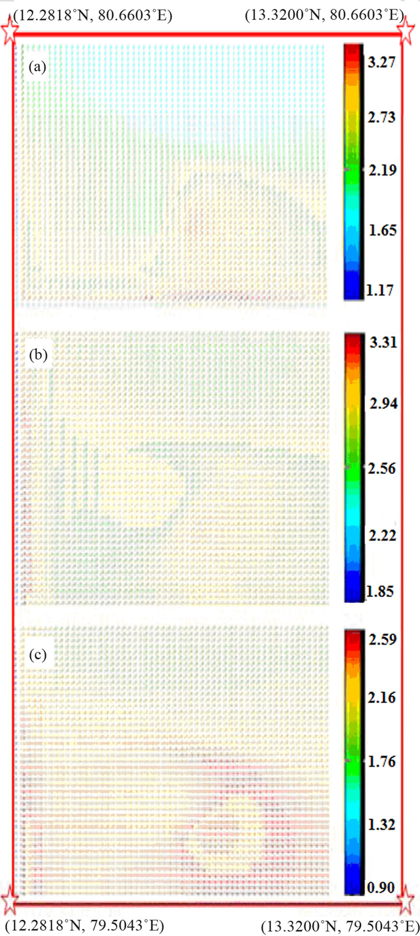
Figure 3. Wind vectors (a) 0100 hours (b) 0300 hours and (c) 0500 hours at 2 m height on 15 September 2010.
z-directions) is 30 × 30 × 12. The grid resolution in xdirection is around 66 m, y-direction is 66 m and in zdirection is about 8 m. The model generated mesodomain wind vectors serve as boundary conditions for the PANACHE-PANEPR CFD model. The model is run on daily basis using the wind solver module. As explained above wind fields will be generated at every time step and hourly wind fields are stored for the analysis. The model generated wind fields at various heights viz. 2, 50 and 100 m at three times in the nighttime (e.g. 0100, 0300 and 0500 LST hours) in the micro domain, and for 2 m height for 15 September 2010, is depicted in Figure 4. At 2 m height, winds are generally coming from SW quadrant at 0100 hours then changed its direction to Westerlies at 0300 hours and finally at 0500 hours they are coming from NW direction (as shown in Figure 4). These figures clearly demonstrate the variation of the wind speed and direction with height as well as with time. Comparatively it is seen that magnitude of the wind is increasing with height. This is a typical wind structure during stable conditions (expected in nighttime), the boundary layer would be capped with higher winds than at the surface. These variations would expect to influence the rate of dispersion of air pollution.
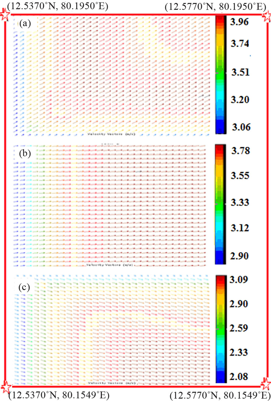
Figure 4. Wind vectors (a) 0100 hours (b) 0300 hours and (c) 0500 hours at 2 m height on 15 September 2010 over IGCAR, Kalpakkam.
4.3. Micro-Scale Dispersion
The micro-scale dispersion of various pollutants over a coastal region of south-east coast of Tamil Nadu has been studied. The micro-scale domain chosen for the present study is depicted in Figure 2. The study region covers a spatial coverage of 4 square kilometers, which contains a varied spatial terrain structures with 94 fields (green), 53 water bodies (deep blue), and 2 urban areas (brown). Dispersion of various pollutants is simulated using dispersion solver of PANACHE. Atmospheric turbulence plays an important role in determining the dispersion. A turbulence model for atmospheric flows needs to capture 1) effects of both shear and thermal characteristics of atmospheric boundary layer and 2) the effects of shear due to obstacles and undulations of the terrain. Keeping in view of this, a turbulence model k - ε is implemented. The k - ε model is a 3D prognostic model that solves an equation for the turbulent kinetic energy and another equation for its dissipation rate [23]. It is suited for all types of flows including flow past obstacles and steeply undulating grounds. This capability of the model that takes care of flow around the obstacles would help in improving the representation of dispersion in the selected urban domain. In the present study, there is no availability of air pollution data (both emission inventory and air quality information). Hence, different scenarios are planned with accidental emissions at two and three locations in the urban set up of micro-scale domain. Three locations are chosen at different land characteristics are given in Figure 2. They are 1) the area of low-rise scattered buildings (named as HEP1 with + sign); 2) high-rise and dense building area (named as HEP2 with * sign) and green field (named as HEP3 with R sign).
Case 1
Numerical experiment has been made to study the dispersion using two arbitrary point sources with steady simulation condition. In the steady simulation solution marches with iterations (cycles) only and the simulation time remains unchanged from the initial defined value. During this type of simulation, following things will not be taken into consideration:
• Duration, Reference time and output dumping time;
• Transient weather data;
• Transient pollutant emissions;
• Time-averaged concentrations.
Two locations with the hypothetical emission inventory are considered, namely HEP1 and HEP2 (Figure 2). These point sources are at an altitude of 10 m from the ground. The concentrations of pollutants at HEP1 for 15 September 2010 at 0100 hour are 60% of Carbon monoxide (CO) and 40% of Sulphur-dioxide (SO2) respecttively with mass flow rate 3 kg·s–1, temperature of 25˚C, release duration of 180 s, and exit velocity of 1.5 ms–1. Similarly, the concentration at location HEP2 are 30% of CO and 70% of SO2 respectively with mass flow rate 2 kg·s–1, temperature of 25˚C, release duration of 180 s with a delay of 2 minutes from the HEP1, and exit velocity of 1 ms–1.
Using the dispersion solver module using the microscale wind field and given emission inventory, the dispersion at various stages of model integration are generated. Basically, these are ground level concentrations and the model implemented in PANACHE only. After 890 iterations the dispersion of CO from the two locations are shown in Figure 5(a). Over the location HEP1 the dispersion is wide spreaded over a large area in comparsion from location HEP2. Similar kind of dispersion pattern is seen in SO2 as well. The release of CO and SO2, at HEP2 was occurred after 2 minutes from HEP1. But that are effect much in terms of dispersion. This could be attributed to the presence of dense urban structures present in HEP2 location. These structures will absorb solar radiation during daytime and release or re-radiate in the nighttime. They act like a secondary source of energy and will generate local thermal regime within the surrounding stable environment. This will generate a local turbulent mixing leading to more dispersion. Even though HEP1 is also an urban setup but with scattered structures, the intensity of reemission of radiation is less compared to HEP2 leads to comparatively less dispersion.
Case 2
In this case, attempt was made to study the dispersion at three arbitrary point sources with unsteady simulation condition. Unsteady simulation solver uses an iterative method to march in time with pre-specified iterations are used to solve the governing equations before proceeding
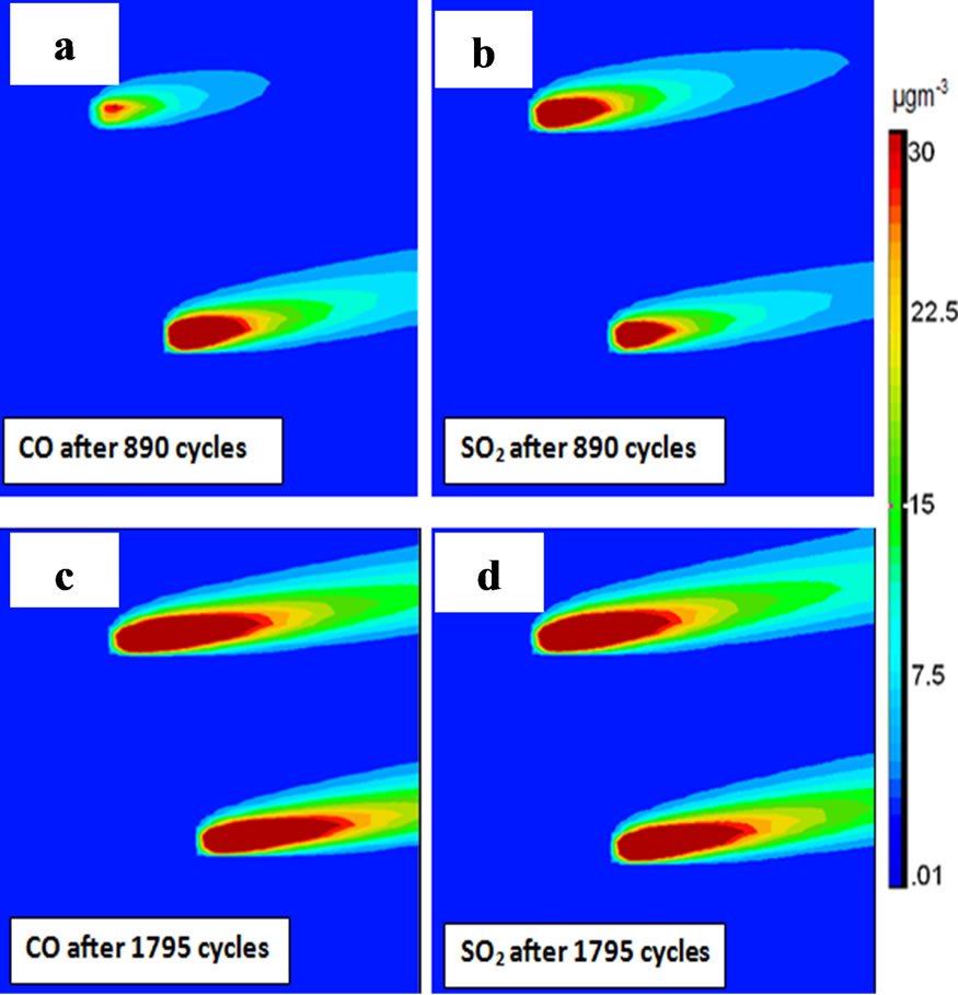
Figure 5. Spatial dispersion of (a) CO after 890 cycles; (b) CO after 1795 cycles; (c) SO2 after 890 cycles; (d) SO2 after 1795 cycles in the steady state simulation mode.
to the next time-step. Three Point sources HEP1, HEP2 and HEP 3 are shown in Figure 2. HEP1 and HEP2 are at an altitude of 10 m and HEP3 is at an altitude of 5 m from the ground. The concentrations of pollutants for 15 September 2010 at 0100 hour at HEP1 are 70% of CO and 30% of Nitrogen (N2) respectively with mass flow rate 2 kg·s–1, temperature of 25˚C, release duration of 120 s, and exit velocity of 2 ms–1. Concentration at HEP2 are 90% of CO and 10% of N2 respectively with mass flow rate 2.5 kg·s–1, temperature of 25˚C, and exit velocity of 2.2 ms–1. The concentration at HEP3 are 50% of CO and 50% of N2 respectively with mass flow rate 1.5 kg·s–1, temperature of 25˚C, release duration of 60 s with a delay of 30 s from HEP1 and HEP2, and exit velocity of 1.8 ms–1. For this case PANACHE is implemented with wind and dispersion solvers which will provide ground level concentrations only. The dispersion of CO and N2 from the three locations are shown in Figure 6. The dispersion over HEP2 is wide spreaded over a large area compared to HEP1 and HEP3 (from 2 minutes 34 seconds to after 8 minutes 54 sec disperison scenario). As explained above (case 1 with two locations), the micro-scale urban setup influence is clearly seen. Interestingly the more rapid dispersion is seen at HEP3 (a open field location—rural in nature). This is due to smaller emission concentrations with very less duration of release compared to the other two locations. This case also clearly signifies the influence of urban setup in dispersion of pollutants in the stable conditions. This kind of dispersion scenarios can not be generated using the Gaussian pollution dispersion models over urban setups.
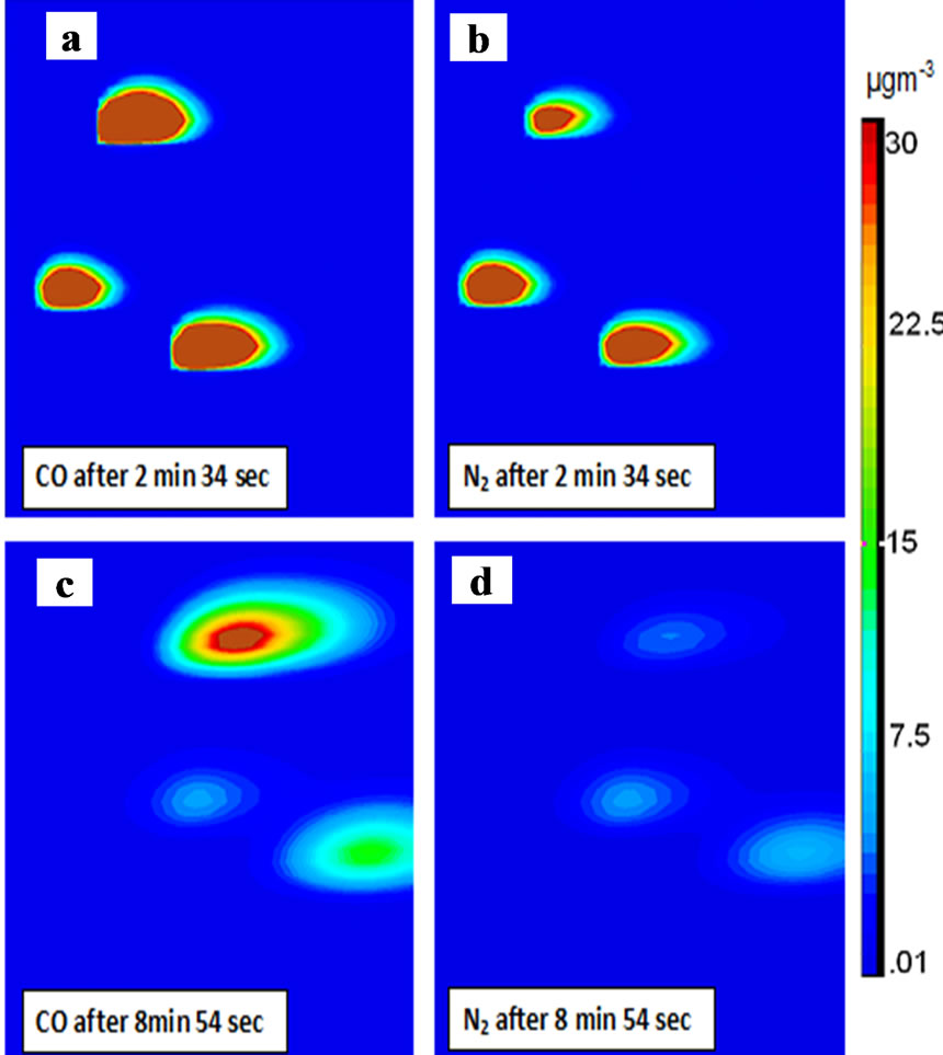
Figure 6. Spatial dispersion of (a) CO after 2 min 34 sec; (b) CO after 8 min 54 sec; (c) N2 after 2 min 34 sec; and (d) N2 after 8 min 54 sec.
Case 3
In this case PANEPR module is implemented to study the dispersion scenarios of three arbitrary sources (as given above) with respect to time at different heights 8, 50 and 100 m. Similar to that of Case 2, wind solver and at HEP1 and HEP2 are at an altitude of 10 m and HEP3 is at an altitude of 5 m from the ground. The concentrations of pollutants for 15 September 2010 at 0100 hour at HEP1 are 70% of CO and 30% of SO2 respectively with mass flow rate 2 kg·s–1, temperature of 25˚C, release duration of 3600 s, and exit velocity of 1.8 ms–1 and concentration at HEP2 are 30% of CO and 70% of SO2 respectively with mass flow rate 2.5 kg·s–1, temperature of 25˚C, release duration of 3600 s and exit velocity of 1.7 ms–1. The concentration at HEP3 are 50% of CO and 50% of SO2 respectively with mass flow rate 1.5 kg·s–1, temperature of 25˚C, release duration of 3600 s, and exit velocity of 2.1 ms–1. The dispersion scenarios generated at these arbitrary sources at different heights for CO and SO2 are given in Figures 7 and 8 respectively. Two specific scenarios are studied one is after 5 minutes 13 seconds and another one after 10 min 54 seconds. Interestingly, both the pollutants completely dispersed and not present at 100 m height of HEP3 location even after 5 minutes 13 seconds. This could be attributed to higher magnitude of wind of the order of 6 ms–1 at those heights are noticed and the emission point is at 5 m height only. But at 8 and 50 m heights after the same time of integration, the dispersion is slightly more spread in HEP2 location compared to HEP1 and HEP3. After 10 minutes and 54 seconds, all the three sources plumes merged together.
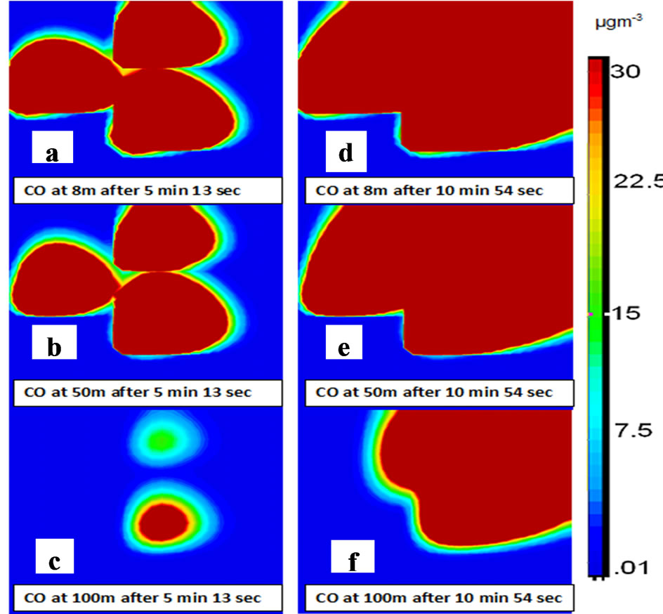
Figure 7. Spatial dispersion of CO (a) after 5 min 13 sec at 8 m height; (b) after 5 min 13 sec at 50 m height; (c) after 5 min 13 sec at 100 m height; (d) after 10 min 54 sec at 8 m height; (e) after 10 min 54 sec at 50 m height; and (f) after 10 min 54 sec at 100 m height.
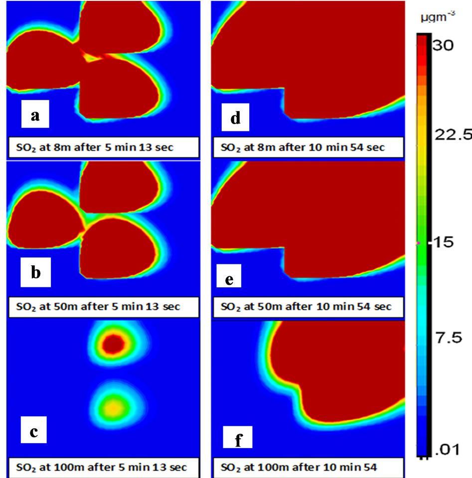
The concentration and spread is more at 8 and 50 m compared to 100 m height. The main purpose of this exercise is to assess the capability of CFD model PANACHE and PANEPR to generate the scenarios for multiple sources of release of any pollutant of known emission inventory and weather information, the dispersion rate with reference to time, space (both horizontal and vertical) for the hazard impact studies. After examining all the above case studies, it is clearly seen that pollution dispersion over urban area is represented well in this CFD model, where Gaussian models does not serve well.
This is due to non representation of turbulent flows and wake flows around the obstacles in Gaussian models where as CFD models can approximate to better accuracy of these turbulent flows and hence with efficient dispersion solver, one can get reasonable picture of pollutant dispersion.
5. Conclusion
Micro-scale dispersion of air pollution over an urban setup in a coastal station in the east coast of India (IGCAR, Kalpakkam) has been studied using a commercial CFD model PANACHE with PANEPR developed by Fluidyn. Winds are generated in the meso-scale domain in the east coast of Tamilnadu, and later these winds are used as boundary conditions to generate the wind field over the urban set up of Kalpakkam region. Locations in the micro-domain (IGCAR, Kalpakkam) with varied land scale such as dense building areas (urban set up), scattered building areas and open fields are selected. Dispersion during stably stratified conditions, i.e. 0100, 0300 and 0500 LST hours during the study period are evaluated. At these locations, hypothetical emission inventories are provided and the CFD model with dispersion module is implemented and various scenarios of pollution dispersion are generated during stably stratified conditions. The dispersion of air pollutants are more over the urban domain due to its reemission of absorbed radiation during daytime. This is significantly changing the thermal structure of the PBL and the mixing which is different from the open fields. The model results also reveal the dispersion of pollutants from individual source can be visualized on horizontal as well as vertical scale with time. This study has given confidence that PANACHE and PANEPR can be used for understanding pollution dispersion by providing actual emission inventories and can be validated reasonably with the available air quality data. The model results suggest that this CFD model has generated reasonable dispersion scenarios over urban scale region which is having profound utility in pollution hazard planning management in major cities and important industrial locations.
6. Acknowledgements
We would like to express our sincere thanks to IGCAR, Kalpakkam providing data of the meteorological towers and Automatic weather stations which was collected during RRE programme, and Fluidyn, Bangalore for providing all facilities and access to use their modeling system in conducting the work. Mr. Srikanth gratefully acknowledges Indian Institute of Technology Kharagpur for providing assistantship to conduct the present study.
REFERENCES
- Y. Anjaneyulu, C. V. Srinivas, D. Hariprasad, L. D. White, J. M. Baham, J. H. Young, R. Hughes, C. Patrick, M. G. Hardy and S. Swanier, “Simulation of Atmospheric Dispersion of Air-Borne Effluent Releases from Point Sources in Mississippi Gulf Coast with Different Meteorological Data,” International Journal of Environmental Research and Public Health, Vol. 6, No. 3, 2009, pp. 1055-1074. doi:10.3390/ijerph6031055
- S. Murakami, R. Ooka, A. Mochida, S. Yoshida and S. Kim, “CFD Analysis of Wind Climate from Human Scale to Urban Scale,” Journal of Wind Engineering and Industrial Aerodynamics, Vol. 81, No. 1-3, 1999, pp. 57-81. doi:10.1016/S0167-6105(99)00009-4
- U. Leenes and A. Pinhas, “The Coastal Boundary Layer and Air Pollution—A High Temporal Resolution Analysis in the East Mediterranean Coast,” Atmospheric Science Journal, Vol. 6, No. 1, 2012, pp. 9-18.
- R. B. Stull, “An Introduction to Boundary Layer Meteorology,” Kluwer Publishers, New York, 1988, p. 666. doi:10.1007/978-94-009-3027-8
- Z. Sorbjan, “Structure of the Atmospheric Boundary Layer,” Prentice-Hall, Upper Saddle River, 1989.
- Venkatram, “Estimating Monin-Obukhov Length in the Stable Boundary Layer for Dispersion Calculations,” Boundary Layer Meteorology, Vol. 19, No. 4, 1980, pp. 481- 485.
- D. B. Turner, “Workbook of Atmospheric Dispersion Estimates: An Introduction to Dispersion Modeling,” 2nd Edition, CRC Press, Boca Raton, 1994.
- M. Holtslag and A. P. Van Ulden, “A Simple Scheme for Daytime Estimates of surface fluxes from Routine Weather Data,” Journal of Climate and Applied Meteorology, Vol. 22, No. 4, 1983, pp. 517-529.
- A. Bass, “Modeling Long-Range Transport and Diffusion,” Proceedings of the 2nd Joint Conference on Applications of Air Pollution Meteorology, New Orleans, 24-27 March 1980, pp. 193-215.
- M. R. Beychok, “Fundamentals of Stack Gas Dispersion,” 4th Edition, 2005, p. 124.
- B. Blocken and J. Carmeliet, “A Review of Wind-Driven Rain Research in Building Science,” Journal of Wind Engineering and Industrial Aerodynamics, Vol. 92, No. 3, 2004, pp. 1079-1130. doi:10.1016/j.jweia.2004.06.003
- G. T. Bitsuamlak, T. Stathopoulos and C. Bedard, “Numerical Evaluation of Wind Flow over Complex Terrain: Review,” Journal of Aerospace Engineering, Vol. 17, No. 4, 2004, pp. 135-145. doi:10.1061/(ASCE)0893-1321(2004)17:4(135)
- R. N. Meroney, “Wind Tunnel and Numerical Simulation of Pollution Dispersion: A Hybrid Approach (Working paper, Croucher Advanced Study Insitute on Wind Tunnel Modeling),” Hong Kong University of Science and Technology, Hong Kong, 2004, p. 60.
- S. Reichrath and T. W. Davies, “Using CFD to Model the Internal Climate of Greenhouses: Past, Present and Future,” Agronomies, Vol. 22, No. 1, 2002, pp. 3-19.
- T. Stathopoulos, “Computational Wind Engineering: Past Achievements and Future Challenges,” Journal of Wind Engineering and Industrial Aerodynamics, Vol. 67-68, 1997, pp. 509-532. doi:10.1016/S0167-6105(97)00097-4
- T. H. Shih, W. W. Liou, A. Shabbir, Z. Yang and J. Zhu, “A New k - ε Eddy Viscosity Model for High: Reynolds Number Turbulent Flows,” Computers & Fluids, Vol. 24, No. 3, 1995, pp. 227-238. doi:10.1016/0045-7930(94)00032-T
- R. Mathur and L. K. Peters, “Adjustment of Wind Fields for Application in Air Pollution Modeling,” Atmospheric Environment, Vol. 24, No. 5, 1990, pp. 1095-1106.
- Fluidyn-PANACHE Technical Manual, 2009.
- B. E. Launder and D. B. Spalding, “Turbulence Models and Their Application to the Prediction of Internal Flows,” Heat and Fluid Flow, Vol. 15, No. 2, 1972, pp. 151-194.
- B. E. Launder and D. B. Spalding, “The Numerical Computation of Turbulent Flows,” Computer Methods in Applied Mechanics and Engineering, Vol. 3, No. 2, 1974, pp. 269- 289. doi:10.1016/0045-7825(74)90029-2
- C. W. Hirt, A. A. Amsden and J. L. Cook, “An Arbitrary Lagrangian-Eulerian Computing Method for All Flow Speeds,” Journal of Computational Physics, Vol. 14, No. 3, 1974, pp. 227-253. doi:10.1016/0021-9991(74)90051-5
- N. R. Meroney, B. M. Leitl, S. Rafailidis and M. Schatzmann, “Wind-Tunnel and Numerical Modeling of Flow and Dispersion about Several Building Shapes,” Journal of Wind Engineering and Industrial Aerodynamics, Vol. 81, No. 1-3, 1999, pp. 333-345. doi:10.1016/S0167-6105(99)00028-8
- G. Mellor and H. J. Herring, “A Survey of the Mean Turbulent Field Closure Models,” AIAA Journal, Vol. 11, No. 5, 1973, pp. 590-599. doi:10.2514/3.6803
NOTES
*Corresponding author.