Journal of Financial Risk Management
Vol.05 No.01(2016), Article ID:65216,14 pages
10.4236/jfrm.2016.51006
Concentration Risk: The Comparison of the Ad-Hoc Approach Indexes
Badreddine Slime, Moez Hammami
1Financial Risk Quant from ENSAE (Ecole Nationale de la Statistique et de l’Administration Economique), Paris, France
2Statistician Economist Engineer at Lunalogic, Paris, France

Copyright © 2016 by authors and Scientific Research Publishing Inc.
This work is licensed under the Creative Commons Attribution International License (CC BY).
http://creativecommons.org/licenses/by/4.0/


Received 29 January 2016; accepted 28 March 2016; published 31 March 2016
ABSTRACT
During the last subprime crisis, the concentration risk issue has become increasingly important in the world of finance. This risk is defined as the loss that we can get from a large exposition of a single name counterparty, a sector or a product. This paper represents some mathematical models for evaluating and quantifying the concentration risk under the Ad-Hoc approaches. This study is based on indexes developed by the theory of inequality and the theory of industrial concentration. This work is about the comparison between these measurements to get which one fits most the financial context. We have selected a set of concentration indexes than we have implemented an empirical test. We propose also a new concentration index. As a result, we shortlist three competitive indexes.
Keywords:
Financial Risk, Credit Risk, Concentration Risk, Concentration Indexes

1. Introduction
The world of finance becomes huge and banks get more and more large exposures without guaranties to hedge some default risks. However, the banks portfolios generate more and more concentration towards counterparties and also sectors. As a result, when the financial system goes into stress then these banks get a big loss and it can drive to the bankruptcy. The main of our issue is the choice of the measurements that can fit most the concentration risk in the financial context.
During the US saving and loan crisis in 1980 more than 1000 institutes had been in default because of the real-estate and energetic sectors concentration. So, most banks of Texas and Oklahoma had got a huge loss due to the debt activities of those sectors. Moreover, in the middle of 90’s and during the real-estate crisis, many of Scandinavian banks had become in bankruptcy situation due to their concentration in this sector. In 2001, German Schmidt Bank had been insolvent and the cause was their concentration of the emergent country.
More recently, the subprime crisis had cost large losses to the financial institutes between 170 billion dollars and the principal reason was their concentration of some product like the Mortgage-Backed Securities and the Collateralized Debt Obligations. The Lehman Brothers was directly after the fall of the MBS/CDOs market in bankruptcy. In the same way, two of the biggest Europeans banks, IKB Deutsche Industries bank and Dexia, cashed a heavy loss. The sovereign crisis in 2010 jeopardized the Dexia bank because of the large concentration of the sovereign debt towards to Greece and Italy.
The concentration risk was discussed the first time as a regulatory issue on the Basel committee in 1999 (BCBS63). It management was reduced to following up the large exposures of the financial institutes and it wasn’t their priorities like the others risks. Therefore, the Basel comities defined the concentration risk as the potential exposure that could be the origin of some large loss into the adverse market conditions. Indeed, the concentration risk could impact both as assets and liability of the bank.
Lutkebohmert (2009) suggests a definition of the concentration risk intothe credit portfolio. So, she defines it as an unequal distribution between the debts exposures under a single counterparty (name concentration) or in many sectors or industries (sector or industry concentration), and there is a strong correlation between this risk and the contagion risk.
Broadly speaking, we can generalize the concept of the concentration risk as the excessive exposure that can be the origin of a big loss according to a single counterparty, a sector, an industry, a product or a risk factor.
The indexes conception for financial purpose is coming from the inequality (Gajdos, 2006; Lubrano, 2014) and the industrial concentration ( Bikker & Haaf 2002 ) theories. In fact, these theories develop some properties that indexes must fulfill. Using these results, Becker, Dullmann, & Pisarek (2004) have listed six properties.
Getting some portfolio with N exposures and denoting that the amount of the i exposure by , with
  defines the total amount exposure of the portfolio. We can define also the share vector of each exposure by
  with
with . The ascending sorted vector of shares (i.e.:
 ) is denoted by
 .
.
The concentration indexes verify  and respect the following properties:
1) Transfert principle: The reduction of an exposure and the increase another higher than the first with the same amount must increase the concentration.
Getting two portfolios  and
and  with:
with:

and , then
 .
.
2) Uniform distribution principle: If all exposures are equal then the concentration is minimal.
Let define a portfolio  and
and .
.
Then .
.
3) Lorentz criterion: If we have two portfolios with the same number of exposures and the sum of the k biggest exposures for the first one is higher than the second one then the concentration indexes follow the same order.
Let’s take two portfolios  and
and , and denote the portfolios with ascending order in shares by
  and
and .
.
If we have , then
 .
.
4) Superadditivity: The fusions of exposures increase the concentration.
Let  a portfolio with N exposures and
  is the regeneration of a second portfolio with
  exposures using the first one with
 , then
 .
.
5) Independence of exposures quantity: If we have a homogenous portfolio with equal shares, then the increasing of the exposures number decrease the concentration indexes.
Let’s have two homogenous portfolios  and
and  with number of exposures N and
  then
then .
.
6) Irrelevance of small exposures: A low additional exposure must not increase the concentration.
Let’s define a portfolio  and
and  is the new exposure verifying
  then
then .
.
With :
: 
Furthermore, the number of exposures doesn’t change in the first three properties contrary to the last three ones. We conclude a relationship between the concentration concept and the number of exposure. However, the properties 1), 2) and 3) come from the inequality theories of revenues. It was mentioned by Lorenz (1905) and Pigou (1912) in their papers, and the aim was about the socials inequalities. The others ones were evoked in industrial concentration context and the purpose was about a monopole issue. Calabrese & Porro (2006) prove that if we have 1) Transfer principal and 6) Irrelevance of small exposures then we have all others properties. Indeed, we get these assertions:
Transfer principle ⇒ 2) Uniform distribution principle
Transfer principle ⇒ 3) Lorentz criterion
Transfer principle and 6) Irrelevance of small exposures ⇒ 4) Superadditivity
Uniform distribution principle et 4) Superadditivity ⇒ 5) Independence of exposures quantity
It must be a link between these properties and the daily transactions upon the exposures to make sense of all these theories. In the other side, they don’t have any use in the concentration concept. In fact, the sixth and the fourth properties give the transaction that could get a credit portfolio. For example, the sell/buy of bonds or the emergence of two or more counterparties. The first one is limited on some risk transfer between two counterparties using some guarantee mechanisms.
The aim of this paper is taking the indexes developed in the inequality and industrial concentration theories and making tests on those to verify the respect of all properties in banking environment.
2. The Most Used Concentration Indexes
Many indexes and ratios were developed to measure the concentration and most of these measurements take the following form:
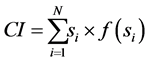
With  is the share of an exposure,
  is the weight of this share and N represents the number of
portfolio exposures. Refer to C. Marfels (1971) , these kinds of concentration measurements were classified by weight form as four classes:
We give 1 to the shares weight values of the k biggest portfolio exposures taking a decreasing sort ( and
and ). As an example we find the concentration ratio.
The weights take the exposures shares as value ( ). The Herfindahl-Hirschman index (HHI) is an example of this family of indexes.
The rank of exposures can represent the weights value, giving an increasing or decreasing sort of the portfolio exposures ( ). We can take as example the Hall-Tidman index (HTI).
The last class weight is a function of shares like a logarithmic function ( ). For example we have the entropy measurement.
Thereafter, we present the most used indexes.
2.1. The Concentration Ratio
The easiest way to conceive a concentration measurement is to calculate the accumulation of the largest exposures under the global exposure of a portfolio. For this we take some portfolio with N exposures and we sort the shares as  with
with . The concentration ratio is defined by:

This ratio verifies the six properties and his implementation is straightforward, however it has a principal drawback: the number k is arbitrary and doesn’t cover the entire distribution of the exposures.
2.2. The Gini Index
The Gini index (Gini, 1921) comes to complete the Lorenz analysis (see annex). This index calculates the deviation according to the perfect repartition. It is defined by the surface between the Lorenz curve and diagonal line. Let’s have a portfolio with N exposures and shares , the numerical formula of the Gini index is:

Broadly speaking, we have the following form in case of a continuous distribution:

When the value of this index is close to 0, then the portfolio isn’t concentrated and all the exposures are equally distributed. Other way, if the value is close to 1 then we have a portfolio extremely concentrated. The Gini index respects the following properties: 1, 2, 3 and 5. So it is independent of the number of exposures because it doesn’t verify the sixth property, but it’s still a complementary tool for analyzing the concentration risk.
2.3. The Hall-Tidman Index (HTI)
This index was developed by Hall & Tidman (1967) for the industrial concentration context. The HTI verifies all of the six properties and the weights get the decreasing rank value of shares. It is defined by the following way:

The relation between this index and the Gini index is:

2.4. The Hannah-Kay Index (HKI)
Hannah & Kay (1977) suggested the following formula to calculate the concentration:

The  parameter gives the elasticity of the weights distribution according to the portfolio composition. This index respects also the six properties of concentration.
2.5. The Herfindahl-Hirschman Index (HHI)
The HHI (Herfindahl, 1950; Hirschmann, 1964) is the most useful index to calculating the concentration and we find it on the macroeconomic empirical studies. This index is equal to the sum of the square shares and it has the following form:

The Herfindahl-Hirschman index verifies the six properties of concentration and it equals to theHKI index for .
.
2.6. The Theil Entropy Index (TEI)
The Theil index (Theil, 1967) is defined as:

This index doesn’t respect the fourth and sixth properties and the relation between TEI and HKI is:

3. The Comparative Study
3.1. The Methodology Presentation
The aim of this study is the implementation of comparative tests between indexes to have the more suitable in the financial context. We define three tests:
Test of the transfer property: this test allows verifying the respect of the transfer property.
Test of the ISE property: the conception of this test allows viewing the behavior of all indexes according to the adding of a small exposure.
Test of the convergence: this test studies the relationship between the concentration indexes and the number of exposures.
These tests will be established on R and under the following assumptions:
The HKI parameter is equal to 3.
The generation of exposures follows the Log-normal distribution.
3.2. Test Results of Ad-Hoc Approach
Test of the transfer property :
This property permits the decrease of portfolio concentration (or the increase of the concentration), in the case of we do some transfers from a high level exposure to a lower level exposure (or in the opposite way to increasing the concentration). This principle is conditioned by respecting the same order between the initial and the final portfolio shares.
First, we generate a portfolio with  exposures following a Log-normal distribution with the mean equal to the 10 and the variance equal to the 3. Then, we sorted it in the increasing order. Thereafter, we proceed to a 1000 transfers from the higher exposures than the fourth quartile to the lower exposures than the second quartile assuring the respect of the initial portfolio order. Then, we calculate the concentration indexes in each iteration. The steps of the processing test are:
1. Generating 1000 exposures following.
2. Sort the exposures in the increasing order.
3. Compute the concentration indexes.
4. Compute the quartiles.
5. Random selection of an exposure lower than the second quartile .
.
6. Random selection of an exposure higher than the fourth quartile .
.
7. Make a transfer of an amount equal to  toward
 .
.
8. Iterate the steps 2 to 7 a 1000 times.
Table 1 summarizes the evolution of the concentration indexes before and after the transfer.
We notice a decreasing of the concentration indexes after a 1000 transfers. Figure 1 visualizes the evolution of these indexes in each transfer iteration.
Figure 2 gives us the allure of the Lorenz curve after and before transfer.
These results show the respect of the first properties for all indexes. Indeed, in each iteration of transfer the concentration indexes decrease on the first graph. Furthermore, the Lorenz curve also respects this property because the surface between the perfect line and the portfolio distribution was reduced after this simulation.
Test of ISE property:
We process in the same way to the last test to implementing the ISE test. Indeed, we generate  exposures with the Log-normal given the mean between 1 and 10, and the variance between 0.3 and 3. Then, we add 1000 new exposures with a 1 as value. The description of the test steps is:
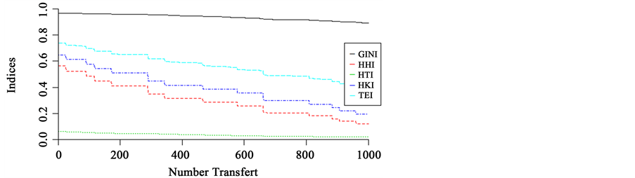
Figure 1. The evolution of the concentration indexes based on the number of exposures.
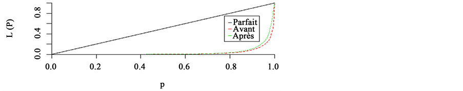
Figure 2. The Lorenz curve before and after transfers.

Table 1. The test transfer results.
1. Initializing the mean and variance value to the 1 and 0.3.
2. Generating a 1000 exposures with the Log-normal (1, 0. 3) distribution.
3. Computing the concentration indexes of the portfolio.
4. Adding an exposure equal to 1.
5. Computing once more the concentration indexes of the new portfolio.
6. Iterating 1000 times the step 4.
7. Increasing the value of the mean with a one unity and the variance with 0.3.
8. Repeating the steps 2 to 5 ten times.
Table 2 summarizes the test results before and after the adding of small exposures.
The impact of the small exposure is insignificant for HHI, HKI and HTI. However, we observe a significant increase on the Gini and theTEI indexes according to the initial portfolio. Figure 3 gives the evolution of indexes in each iteration of the adding.
Figure 4 illustrates the concentration indexes in 3D based on the distribution parameters.
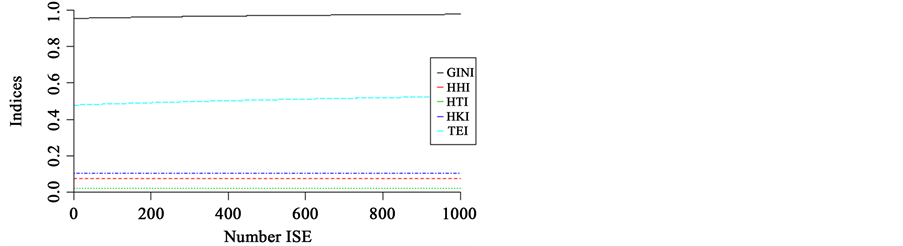
Figure 3. The concentration indexes evolution based on the number of the adding.
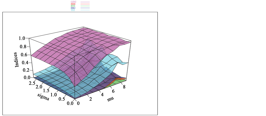
Figure 4.The surface of the test ISE based on the Log-normal parameters.
Table 2. The test ISE results.
Giving these results, Only HHI, HKI and HTI respect the sixth property. On the other side, both Gini and TEI don’t verify this property. In fact, the increase of exposures number should decrease the concentration; contrariwise we get the opposite effect in the inequality theory. Besides that, the Gini and TEI were developed for measuring the inequalities, and then they must have an opposite effect according to the sixth property.
The test of the convergence :
This test defines a new property to analyze the evolution between the concentration indexes and the number of exposures. Indeed, the portfolio granularity is characterized by a number of exposures higher enough such as makes the idiosyncratic risk vanish. According to this result, we can conclude that portfolios with a very higher number of exposures should be less concentrated than those with a lower number of exposures. The purpose of this test is to verify amongst of which indexes respect this result.
The implementation of this test is based on generating of one million of the exposures with the Log-normal distribution, and we randomly select 50 portfolios with n exposures between 2 and 1000. We calculate in each iteration the mean and the variance of the concentration indexes for these portfolios. The steps processing of this test are:
1) Generating 106 exposures following the Log-normal (10, 3) distribution.
2) Initializing the number of exposure to .
.
3) Selecting 50 portfolios with  exposures.
4) Computing the concentration indexes of each portfolio.
5) Computing the mean and the variance of all portfolios concentration indexes.
6) Incrementing the number of exposures by 1.
7) Iterating 1000 times the steps 3 to 6.
Table 3 gives means and variances of concentration indexes with two and one thousand exposures.
Figure 5 shows the evolution of the mean concentration indexes according to the number of the exposures.
Giving this graph, we notice that HHI, HKI and HTI decrease according to the number of exposures. On the other side, the Gini index increases based on the number of exposures. Moreover, the TEI index has a stagnating trend. We also conclude that all indexes become constant for higher levels of number of exposures.
3.3. Recapitulation
Table 4 summarizes the indexes formula of the concentration indexes with some drawbacks:
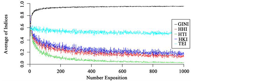
Figure 5. The evolution of the concentration indexes based on the number of the exposures.
Table 3. The convergence test results.
Table 4. The concentration indexes summarize.
4. The Index Proposal: The Hammami-Slime Index (HSI)
We will try in this section to make a suggestion of an index, in one hand, to calculate the portfolio concentration taking account to the banking environment, and on the other hand, to keep the relationship with the number of exposures. This index includes an  parameter allowing the adjustment of the concentration according to the number of exposures in the portfolio. In fact, if we have one exposure then the concentration is maximal and equal to 1 for HHI, HTI and HKI. This result is still logical with the concentration concept. But, if we go to two exposures for a homogeneous portfolio the concentration indexes become 0.5. It means that the concentration is divided by two, however the portfolio is still always very concentrate and the index must have a very higher value. The new index will adjust the discrepancy over the number of exposures. The index is defined by:

If  then the index is equal to
 .
.
Furthermore, if , then
 . This index verifies the six properties (see annex). The HSI index is less complex than the HKI and the relationship between both of these indexes is:

Figure 6 illustrates the evolution of the concentration according to the number of exposures and the α parameter in case of homogeneous portfolio.
We find that the convexity of the concentration decreases on α for a homogeneous portfolio. So, this parameter gives importance to the concentration according to the number of exposures. Indeed, if we have  then the concentration goes from 1 to 0.84 for some portfolios with two exposures in case of the homogeneous portfolio. This parameter can take the adjustment role of the concentration indexes according to the number of exposures. This index gives a coherent quantification for portfolios with a small number of exposures than the other indexes. The convergence test confirms this property also for inhomogeneous portfolios. Figure 7 gives us the test results:
5. Conclusion and Future Directions
Gini and TEI indexes didn’t verify the six properties unlike the other indexes. For these results we implemented
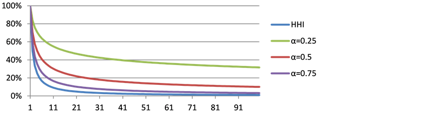
Figure 6. The concentration curve based on the number of exposures and α.
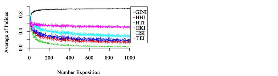
Figure 7. The comparison between the evolution of HSI and the others indexes based on number of exposures.
the tests of the first and the sixth properties.
At the end, we got four concurrent indexes and we couldn’t have more flexibility to reduce this list. So, we added a new test to study the evolution of these indexes according to the number of exposures. We concluded that the HTI index tended to zero faster than the others. Indeed, it couldn’t give a good measurement of portfolios with a small number of exposures.
These tests on the concentration indexes enabled us to choose among the most suitable to the financial context. We retained the following indexes: HHI, HKI and HSI. Furthermore, the HSI index gave a more consistent measurement of portfolios with a small number of exposures.
The Ad-Hoc approach was sample to implement and we could have a global view of the concentration risk. However, this approach did not take into consideration de specific risk factors like the PD and LGD. On the other hand, it did not allow computing the provision charge of capital requirement to cover the concentration risk. For these raisons, the Add-On approach came to underpin the first approach and to complete these gaps.
Cite this paper
Badreddine Slime,Moez Hammami, (2016) Concentration Risk: The Comparison of the Ad-Hoc Approach Indexes. Journal of Financial Risk Management,05,43-56. doi: 10.4236/jfrm.2016.51006
References
- 1. Basel Committee on Banking Supervision (1999).
http://www.bis.org/publ/bcbs63.pdf - 2. Becker, S., Dullmann, K., & Pisarek, V. (2004). Measurement of Concentration Risk—A Theoretical Comparison of Selected Concentration Indices, Unpublished Working Paper, Deutsche Bundesbank.
- 3. Bikker, J. A., & Haaf, K. (2002). Measures of Competition and Concentration in the Banking Industry: A Review of Literature. Netherland: Central Bank of the Netherlands.
- 4. Calabrese, R., & Porro, F. (2006). Single-Name: Concentration Risk in Credit Portfolios: A Comparison of Concentration Indexes. Monthly Report, Deutsche Bundesbank.
- 5. Gajdos, T. (2006). Les fondements axiomatiques de la mesure normative des inégalités. HAL.
- 6. Gini, C. (1921). Measurement of Inequality of Incomes. Economic Journal, 31, 124-126.
http://dx.doi.org/10.2307/2223319 - 7. Hall, M., & Tideman (1967). Measures of Concentration. Journal of American Statistical Society, 62, 162-168.
http://dx.doi.org/10.1080/01621459.1967.10482897 - 8. Hannah, L., & Kay, J. A. (1977). Concentration in Modern Industry. London: Mac Millan Press.
http://dx.doi.org/10.1007/978-1-349-02773-6 - 9. Herfindahl, O. (1950). Concentration in the U.S. Steel Industry, Dissertion. New York: Columbia University.
- 10. Hirschmann, A. (1964). The Paternity of an Index. American Economic Review, 54, 761.
- 11. Lorenz, M. O. (1905). Methods of Measuring the Concentration of Wealth. Publications of the American Statistical Association, 9, 209-219.
http://dx.doi.org/10.2307/2276207 - 12. Lubrano, M. (2014). The Econometrics of Inequality and Poverty.
- 13. Lutkebohmert, E. (2009). Concentration Risk in Credit Portfolios. Berlin: Springer-Verlag.
- 14. Marfels, C. (1971). Absolute and Relative Measures of Concentration Reconsidered. Halifax: Kyklos.
http://dx.doi.org/10.1111/j.1467-6435.1971.tb00631.x - 15. Theil, H. (1967). Economics and Information Theory. North Holland: Amsterdam.
Appendix
The Lorenz curve:
The Lorenz curve doesn’t give one concentration index and a unique ranking of concentration between two portfolios, but it gives a global view according to the perfect diversification. It defines a cumulative percentile of exposures sizes. Let’s a set of exposure such as , then The Lorenz curve is defined by:
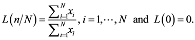
Given a continuous distribution f and it distribution function F invertible with finite mean, then The Lorenz curve becomes:

The perfect concentration is given by , and the concentration of Log-normal distribution is equal to:

With  is the cumulative function of a Gaussian distribution.
The following graph gives an example of the Lorenz curve of a Log-normal distribution:
Proof of concentration properties respect for the HSI index:
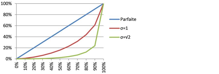
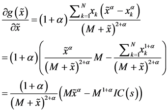
Let’s have two portfolios s and  verifying the conditions of the first property, we define the following function:
The function  is continuous, and
 . The derivative of this function according to is:

Then 
In the same way, we can demonstrate the sixth property defining two portfolios verifying the conditions of this property, and the following function  such as:

This function is continuous and . The derivative according to
  is equal:


We conclude the following result , and also
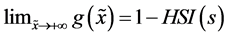 . Otherwise we get
 . The necessary condition to have
  (the property 6 is verified) is
 .
.
The minimum of this function is equal to:
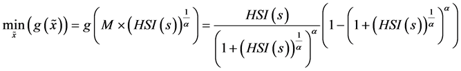
With 
In order to complete this study, we calculate the roots of :


In case of the HHI index , we get the following solutions of the last equation:

As a conclusion, the g function becomes positive beyond an adding upper than . The second root gives us the magnitude order of the new exposure to increase the concentration. So, if we have the concentration index of some portfolio closer than 1, then we need many adds to reduce the concentration because we have the follow-
ing assertion: . Indeed, the concentration couldn’t increase because in the practice there are limits of the operations amount.
On the other side, if a portfolio has a minimal concentration in other word exposures are equiponderant, then it will be very sensitive to the concentration and some small adding could increase the concentration because we
have . To study the impact of the small exposure in terms of concentration, let’s have a portfolio with Log-normal distribution.
In our case, the portfolio is characterized by:
The figure illustrates the evolution of  for
for :
:
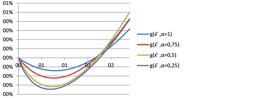
The table gives the roots and also the abscissas where this function changes the sign:
Therefore, the concentration will increase in the case of , and we also notice that all roots are bigger than the maximum of exposures. So as we know, in the real life we can’t have this kind of operation to obtain the last condition. On the other hand, as we see the concentration increases on , the same applies to the root which explains the adjustment of the concentration in relation to the overall structure of the portfolio.