American Journal of Climate Change
Vol.2 No.2(2013), Article ID:33510,9 pages DOI:10.4236/ajcc.2013.22014
Global River Basin Modeling and Contaminant Transport
Center for Water Science and Engineering, Science Applications International Corporation, McLean, USA
Email: samuelsw@saic.com
Copyright © 2013 Rakesh Bahadur et al. This is an open access article distributed under the Creative Commons Attribution License, which permits unrestricted use, distribution, and reproduction in any medium, provided the original work is properly cited.
Received January 4, 2013; revised February 6, 2013; accepted February 15, 2013
Keywords: Hydrology; Geographic Information Systems; Surface Water
ABSTRACT
Using geographic information system techniques, elevation derived datasets such as flow accumulation, flow direction, hillsope and flow length were used to delineate river basin boundaries and networks. These datasets included both HYDRO1K (based on 1 km resolution DEM) and HydroSHEDs (based on 100 meter Shuttle Radar Topography Mission). Additional spatial data processing of global landuse and soil type data were used to derive grids representing soil depth, texture, hydraulic conductivity, water holding capacity, and curve number. These grids were input to the Geospatial Stream Flow model to calculate overland flow (both travel time and velocity). The model was applied to river basins across several continents to calculate river discharge and velocity based on the use of satellite derived rainfall estimates, numerical weather forecast fields, and geographic data sets describing the land surface. Model output was compared to historical stream gauge observations as a validation step. The stream networks with associated discharge and velocity are used as input to a riverine water contamination model.
1. Introduction
Modeling the fate and transport of waterborne contaminants in rivers and watersheds requires fundamental knowledge of the hydrologic cycle. The processes are well known and hydrologic models have been developed. The limiting factor in applying these models is the underlying data. Data sources for rivers and watersheds in the United States have been integrated with models [1-5] to simulate both deliberate and accidental releases. However, for applications outside the US, little or no waterborne modeling has been done for chemical, biological or radiological constituents.
The physical processes involved in watershed analysis start with the deposition of water on the earth’s surface as rain or snow. The liquid water (including snow melt) then moves over the surface forced by gravity to seek the lowest point in the terrain. As the liquid flows over the surface, some of it percolates into the soil. The fraction going into the soil depends on the land cover, soil texture and saturation, which in turn depends on the rate at which the soil dries out due to evapotranspiration.
The application of transport models is dependent on the availability of data to implement the modeling and to verify model fidelity. To apply complex models to watersheds, simplification and adaptation are necessary to address the complexity of each individual modeling domain. For a given setting, some terms in the governing equations are less important than others, allowing simplification and a more efficient implementation. However, over-simplification can result in simulation models that are far removed from the physical, chemical, or biological characteristics of water bodies.
Global river flows are an important input (boundary condition) to estuarine, coastal and oceanic models. Real-time river flow [6] is also a critical input to river models used to portray transport and dispersion of toxic contaminants released deliberately or accidentally onshore. In the absence of a network of real-time river gages, as is available in the US, alternative means are required for calculating the flow of drainage streams and rivers.
Two models (GeoSFM and ICWater) were used, respectively, to create drainage networks (with associated flows and velocities) and to perform contaminant transport based on these networks. The GeoSFM processes and datasets are described in section 2 below. The application of ICWater for downstream contaminant transport and dispersion is discussed in Section 4.
2. Hydrologic Data Processing
In this study, the first step in the process was to assemble hydrologic and terrain data sets from remotely sensed data. This includes: digital elevation model, land use, soils, catchment boundaries, stream network, precipitation, and evapotranspiration. Parameterization of the basins’ hydrologic properties is accomplished through the use of three data sets describing the surface topography, land cover, and soils. In addition, literature searches are performed to gather additional hydrologic data to fill data gaps (this may yield additional local data that can be used to enhance the digital datasets and to perform model calibration). Once this process is complete, river discharge is calculated using hydrologic modeling techniques within the GeoSpatial Stream Flow Model (GeoSFM) (Figure 1).
The USGS [7,8] developed GeoSFM, which makes use of terrain, vegetative cover, soil absorption characteristics, precipitation and evapotranspiration data to calculate river flow. Much of the input data for GeoSFM are derived from satellite observations. The GeoSFM has been applied successfully in a portion of Africa [9,10] using HYDRO1K [11]. In recent applications [12], HYDRO1K has been replaced by HydroSHEDS, a higher resolution stream network [13].
HydroSHEDS is derived from elevation data of the Shuttle Radar Topography Mission (SRTM) at 3 arcsecond resolution. The original SRTM data have been hydrologically conditioned using a sequence of automated procedures. Existing methods of data enhancement and newly developed algorithms have been applied, including void-filling, filtering, stream burning, and upscaling techniques. Manual corrections were made where necessary. Preliminary quality assessments indicate that the resolution of HydroSHEDS significantly exceeds that
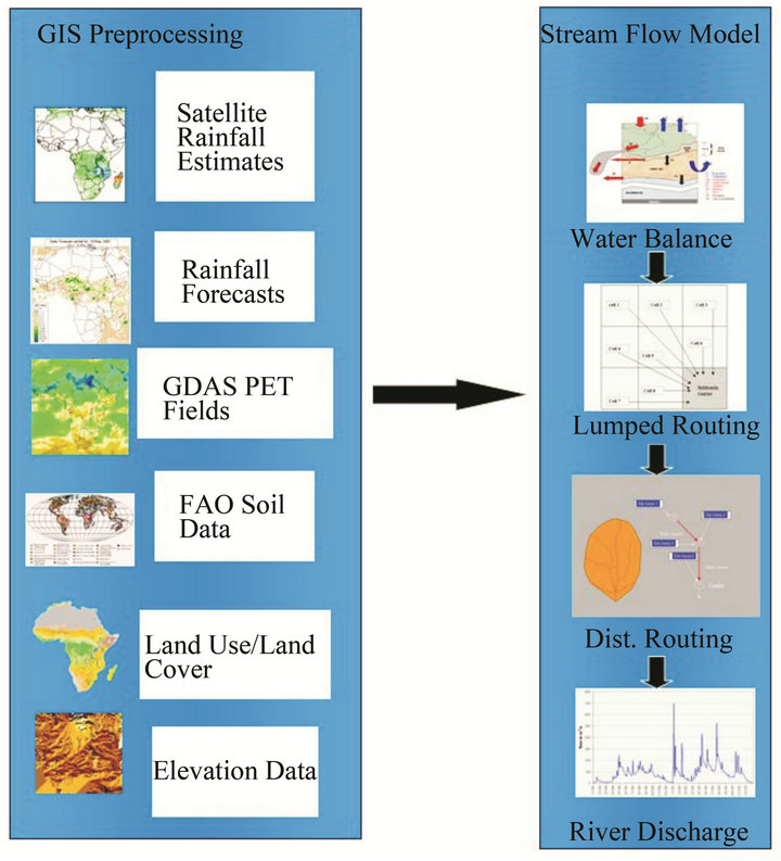
Figure 1. GeoSFM data sets and processing steps [7].
of existing global watershed and river maps [13]. HydroSHEDS vector and raster datasets include: stream networks, watershed boundaries, drainage directions, and ancillary data layers such as flow accumulations, distances, and river topology information.
The Digital Soil Map of the World [14] was derived from an original compilation at 1:5,000,000 scale. Attributes for the soil associations are used to set hydraulic parameters that govern interflow, soil moisture content, and deep percolation to the ground water table. Rates at which subsurface layers release water to the stream network also depend on these physical soil attributes. Global Land Use/Land Cover was provided by the USGS [15].
Daily precipitation is obtained from the National Oceanic and Atmospheric and Administration (NOAA) Climate Prediction Center Morphing technique (CMORPH) [16]. CMORPH produces global precipitation analyses at very high spatial and temporal resolutions. This technique uses precipitation estimates that have been derived exclusively from low Earth orbit satellite microwave observations, and whose features are transported via spatial propagation information that is obtained entirely from geostationary satellite IR data. CMORPH is not a precipitation estimation algorithm but a means by which estimates from existing microwave rainfall algorithms can be combined. Therefore, this method is extremely flexible such that any precipitation estimates from any microwave satellite source can be incorporated. CMORPH data is available in GIS format on a 1/4 × 1/4 degree grid.
Daily net precipitation and evapotranspiration (PET) data is also obtained from the USGS Global Data Assimilation System. PET is the maximum extraction rate from soil and is based on air temperature, atmospheric pressure, wind speed, relative humidity, and solar radiation (long wave, short wave, outgoing and incoming). The daily PET is calculated on a spatial basis using the Penman-Monteith equation and the formulation of Shuttleworth [17]. GeoSFM converts PET to actual daily evapotranspiration based on antecedent soil moisture conditions. PET is available on a 1 × 1 degree grid [18].
3. River Basin Modeling Results
For this project, six river basins (Danube, Dneister, KuraAraks, Yangtze, Hwang he and Mekong) were selected as case studies (Figure 2). The river basin boundaries are based on two datasets: a revised version of the Major Watersheds of the World dataset-distributed through the International Water Management Institute [19] and the EROS Data Center HYDRO1K basin boundaries developed at the US Geological Survey [11]. River basin boundaries were digitally derived using ETOPO5, 5- minute gridded elevation data, and known locations of
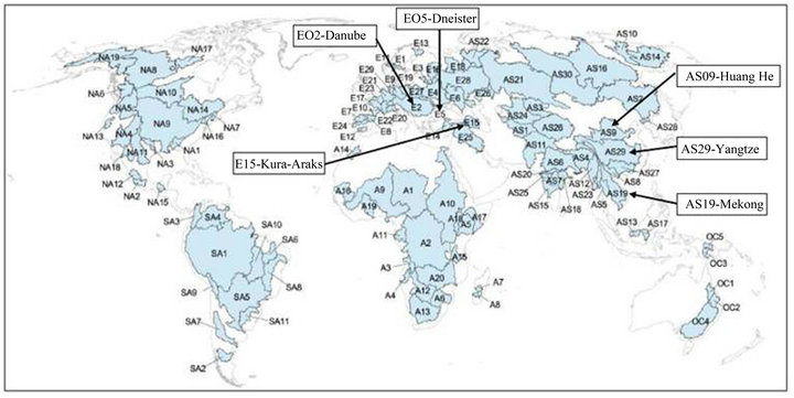
Figure 2. Major river basins of the world and the six case study basins [21].
rivers. The HYDRO1K is a geographic database derived from the USGS’ 30 arc-second digital elevation model of the world, GTOPO30. The results of the stream delineation for the Dneister River Basin are shown in Figure 3. Observed [21] and simulated peak and annual average flows at the mouth of the Dneister are in good agreement as shown in Table 1. Similar results [22] are presented for the Kura-Araks basin (Figure 4 and Table 2).
The basin map for the Mekong River is shown in Figure 5. The average flow from nine gauging stations was obtained from the Mekong River Commission [23] for use in comparing observed and simulated flows. This comparison of averaged observed and simulated flows is tabulated in Table 3. Although not shown in this paper, similar river delineations and flow comparisons were made for the Danube, Yangtze and Hwang He basins.
4. Riverine Contamination Modeling
The output of GeoSFM can serve as input to the Incident Command Tool for Drinking Water protection (ICWater). ICWater was developed with the RiverSpill modeling tool [24] as the hydrological engine. The RiverSpill system allows the user to track a chemical or biological agent, under real-time flow conditions, from the point of introduction to downstream water supply intakes. It determines the concentration and decay rate of an agent as it is dispersed within the water and identifies the population served by the water system that may be at risk. ICWater integrates multiple sources of information to give decision makers concise summaries of current conditions and forecasts of future consequences of contami-
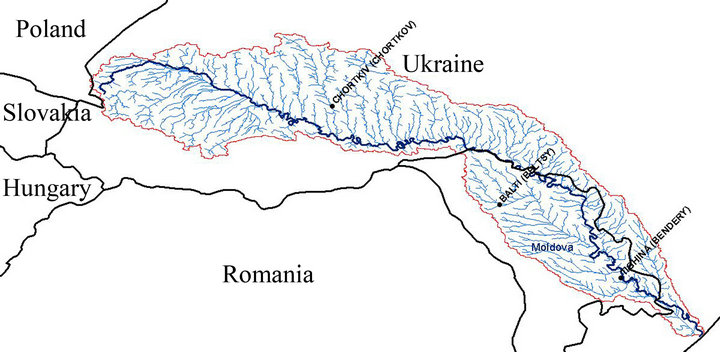
Figure 3. Map of the Dneister River Basin.
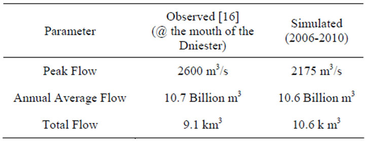
Table 1. Comparison of observed [21] and simulated flows for the Dneister River Basin.
nated public water supplies. The time-dependent distribution of contaminant concentrations, simulated by modeled dispersion, dilution and substance decay, is reported for contaminants arriving at drinking water intakes. Figure 6 shows the current functionality in ICWater.
ICWater calculates the downstream concentration using the dispersion equation to create the downstream trace. Runoff is incorporated into the downstream calculation based on deposition from an atmospheric transport/dispersion model or user input. Runoff from atmos-
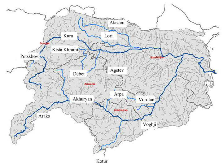
Figure 4. Map of the Kura-Araks River basin.
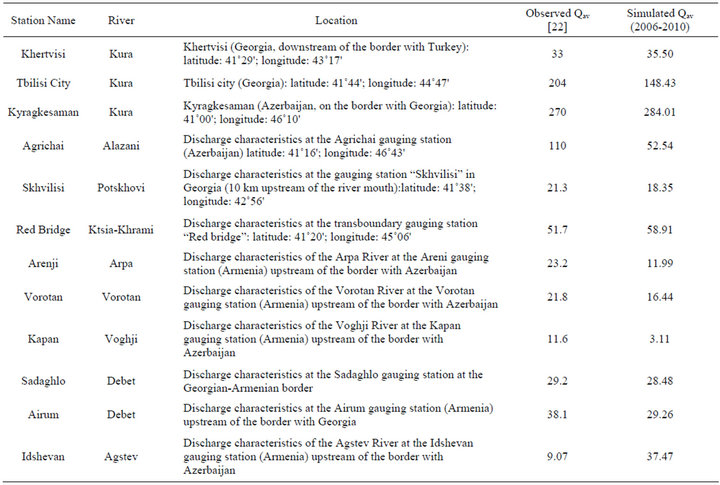
Table 2. Comparison of observed [22] and simulated flows for the Kura-Araks River Basin.
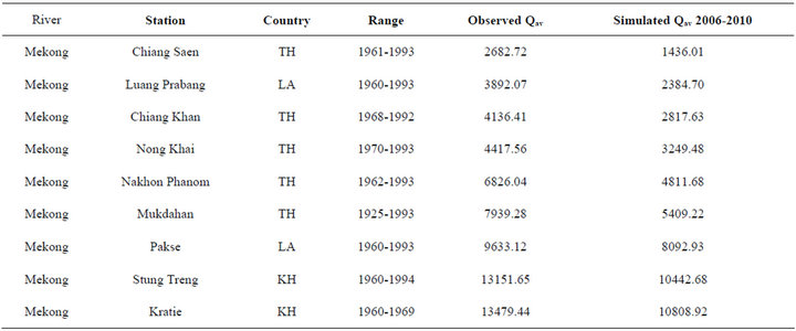
Table 3. Comparison of observed [23] and simulated flows for the Mekong River Basin.
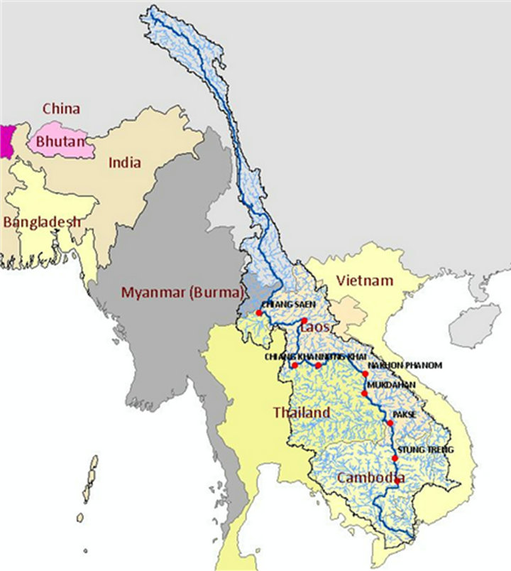
Figure 5. Map of the Mekong River Basin.
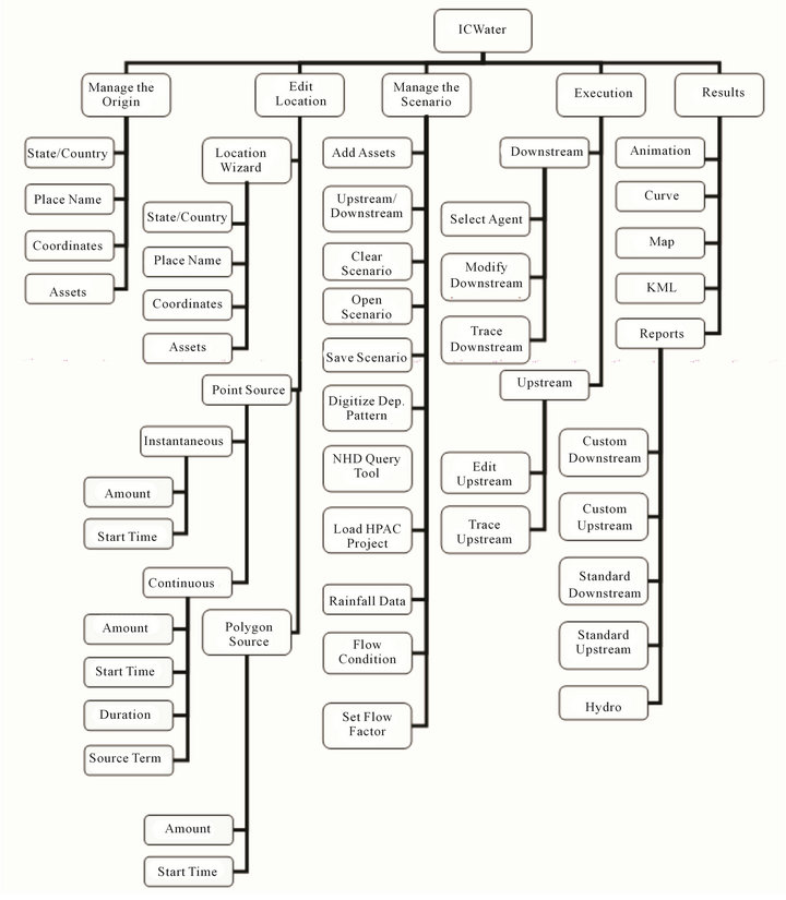
Figure 6. ICWater functionality for riverine contaminant transport modeling.
pheric deposition of contaminants is modeled as nonpoint source pollution. For non-point source pollution, CMORPH rainfall data are used to calculate runoff of contamination from the land surface to the receiving stream. The dispersion equation used in ICWater characterizes one-dimensional turbulent diffusion in constant density flow. The concentration is considered to be a function only of time and distance along the longitudinal axis. Reach velocities, estimated from real-time measurements reported from stream gauging stations, are applied over the uniform cross sections along a reach (defined from confluence to confluence). Substance decay is modeled as a first order exponential process.
A case study for a toxic chemical spill in the Danube River basin is shown in Figure 7. On January 30th 2000, the dam containing toxic waste material from the Baia Mare Aurul gold mine in North Western Romania burst and released 100,000 cubic meters of waste water, heavily contaminated with cyanide, into the Lapus and some tributaries of the river Tisza, one of the biggest in Hungary [25-27]. The cyanide concentration at the accident site was 7800 mg/l. ICWater was run with this source term and the results are shown in Figure 8. On February 4, the cyanide concentration at Szeged, Hungary was reported to be 1.1 mg/l. The model predicted the concentration to be 1.25 mg/l. After sixteen days, the concentration in the Danube River as measured at 0.06 mg/l (the model prediction was 0.1 mg/l).
5. Summary and Conclusions
This approach for watersheds and rivers uses the GeoSpatial Stream Flow Model to generate river networks, catchments, flows and velocities for input to the Incident
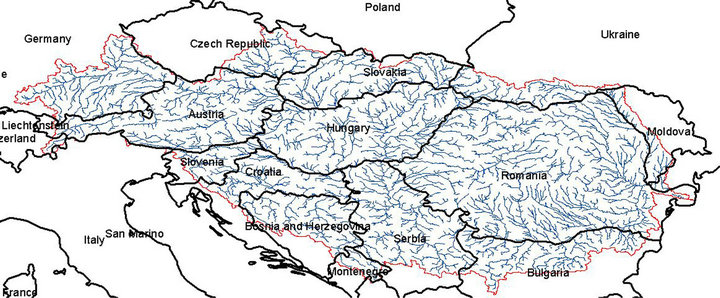
Figure 7. Map of the Danube River Basin.
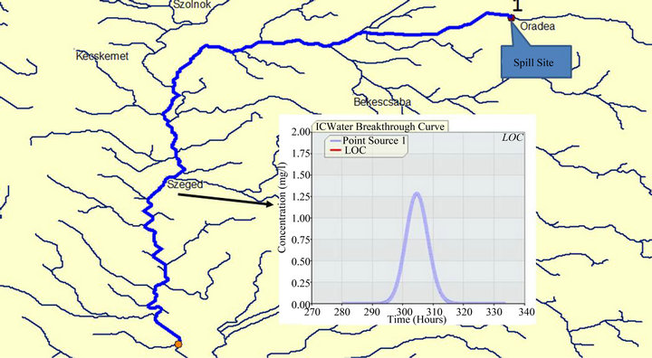
Figure 8. ICWater simulation (downstream trace) of cyanide spill in the Danube River Basin.
Command Tool for Drinking Water Protection toxic spill model. The process followed is:
• Prepare the input data for GeoSFM from a set of global databases (terrain, land use, soils, rainfall, and evapotranspiration).
• Organize and integrate the input databases so that the specification of an area of interest triggers the extraction of data to run the model.
• Automate Hydrology Data Extraction based on Polygon of Interest.
• Run GeoSFM
• Calibrate and validate the flow/velocities with observed data from the Global Runoff Data Center database or any other set of available observations.
• For the contaminant transport specify an area of interest; extract the river network, catchments, flows, velocities and assets and import to ICWater.
• Run the ICWater model to predict downstream time of travel and concentration of toxic spills.
There are requirements for quantified river flow to support the prediction and analyses of contaminant transport and dispersion worldwide. Procedures have been developed for use throughout the US which rely on the existing network of real-time gages. In many parts of the world there are few or no real-time river gages or the gage observations may not be accessible. A capability for determining global river flows has been developed by integrating HydroSHEDS with GeoSFM to calculate river discharge in regions with few or no stream gauges or other databases describing river networks and catchments. Atmospheric forcing is provided by satellite derived global forecasts of rainfall and evapotranspiration. A contaminant transport application has been validated against a chemical spill in the Danube River Basin.
The architectural framework in ICWater relies on the Environmental Systems Research Institute, Inc.’s Geographic Information System and various interface modules have been created to enable the seamless and transparent communication of the software components with the common map background and with the databases. ICWater operates as an extension to ArcGIS or as a stand-alone code using the ArcGIS Engine runtime libraries.
6. Acknowledgements
This project was supported by a contract to Science Applications International Corporation from the US Department of Defense.
REFERENCES
- C. R. Horn, S. A. Hanson and L. D. McKay, “History of the US EPA’s River Reach File: A National Hydrographic Database Available for ARC/INFO Applications,” 1994. www.epa.gov/waters/doc/historyrf.pdf
- C. R. Horn and W. M. Grayman, “Water Quality Modeling with the EPA Reach File System,” Journal Water Resources Planning and Management, Vol. 119, No. 2, 1993, pp. 262-274. doi:10.1061/(ASCE)0733-9496(1993)119:2(262)
- D. R. Maidment, “Arc Hydro GIS for Water Resources,” ESRI Press, Redlands, 2002.
- B. DeVantier and A. Feldman,”Review of GIS Applications in Hydrologic Modeling,” Journal Water Resources Planning Management, Vol. 119, No. 2, 1993, pp. 246- 261. doi:10.1061/(ASCE)0733-9496(1993)119:2(246)
- W. B. Samuels, and D. Ryan, “ICWater: Incident Command Tool for Protecting Drinking Water,” Proceedings ESRI International User Conference, San Diego, 25-29 July 2005.
- GTN-R, “Global Terrestrial Network for River Discharge (GTN-R),” 2007. http://www.bafg.de/GRDC/EN/04_spcldtbss/44_GTNR/gtnr_node.html
- K. O. Asante, G. A. Artan, S. Pervez, C. Bandaragoda and J. P. Verdin, “Technical Manual for the Geospatial Stream Flow Model (GeoSFM): US Geological Survey Open-File Report 2007-1441,” US Geological Survey, Reston, 2008, p. 65
- G. Artan, J. Verdin and K. Asante, “A Wide-Area Flood Risk Monitoring Model,” Proceedings of the Fifth International Workshop on Application of Remote Sensing in Hydrology, Montpellier, 2-5 October 2001.
- J. P. Pickus, J. Johnson, M. Chehata, R. Bahadur, D. E. Amstutz and W. B. Samuels, “Development of a Global River Transport and Observation Network,” Proceedings AWRA GIS Specialty Conference, San Mateo, 17-19 March 2008.
- K. O. Asante, R. D. Macuacua, G. A. Artan, R. W. Lietzow and J. P. Verdin, “Developing a Flood Monitoring System from Remotely Sensed Data for the Limpopo Basin,” IEEE Transactions on Geoscience and Remote Sensing, Vol. 45, No. 6, 2007, pp. 1709-1714. doi:10.1109/TGRS.2006.883147
- USGS, “HYDRO1K Elevation Derivative Database,” 2006. http://eros.usgs.gov/products/elevation/gtopo30/hydro/index.html
- W. B. Samuels and D. E. Amstutz, “Using HydroSHEDS and GeoSFM to Calculate River Discharge,” Proceedings International Perspective on Environmental and Water Resources, Bangkok, 5-7 January 2009.
- WWF, “HydroSHEDS Overview,” 2007. http://www.worldwildlife.org/hydrosheds
- FAO, “Digital Soil Map of the World and Derived Properties on CD-ROM,” 1997. http://www.fao.org/AG/agl/agll/dsmw.htm
- USGS, “Global Land Cover Characterization (GLCC),” 2006. http://eros.usgs.gov/products/landcover/glcc.html
- R. J. Joyce, J. E. Janowiak, P. A. Arkin and P. Xie, “CMORPH: A Method that Produces Global Precipitation Estimates from Passive Microwave and Infrared Data at High Spatial and Temporal Resolution,” Journal Hydrometeorology, Vol. 5, 2007, pp. 487-503. doi:10.1175/1525-7541(2004)005<0487:CAMTPG>2.0.CO;2
- W. J. Shuttleworth, “Evaporation,” In: D. Maidment, Ed., Handbook of Hydrology, McGraw-Hill, Inc. New York, 1992.
- USGS, “Global Potential Evapotranspiration (PET),” 2007. http://earlywarning.usgs.gov/adds/global/web/imgbrowsc2.php?extent=glpt
- WMI, “Major watersheds of the world,” 2003. http://www.wri.org/publication/watersheds-of-the-world
- WRI, “Major watersheds of the world,” 2003. http://pdf.wri.org/watersheds_2003/gm1.pdf
- OSCE/UNECE, “Transboundary Diagnostic Study for the Dniester River Basin,” Environment, Housing and Land Management Division, United Nations Economic Commission for Europe, November 2005.
- ECONOMIC COMMISSION FOR EUROPE, “Convention on the Protection and Use of Transboundary Watercourses and International Lakes. Our Waters: Joining Hands Across Borders,” First Assessment of Transboundary Rivers, Lakes and Groundwaters, 2007. http://www.unece.org/fileadmin/DAM/env/water/blanks/assessment/assessment_full.pdf
- Mekong River Commission, “Overview of the Hydrology of the Mekong Basin,” Mekong River Commission, Vientiane, November 2005, p. 73.
- W. B. Samuels, D. E. Amstutz, R. Bahadur and J. M. Pickus, “RiverSpill: A National Application for Drinking Water Protection,” Journal of Hydraulic Engineering. Vol. 132, No. 4, 2006, pp. 393-403. doi:10.1061/(ASCE)0733-9429(2006)132:4(393)
- Independent of UK, “Cyanide Leak Heads towards Danube Killing Every Living Thing in Its Path,” 2000. http://www.commondreams.org/headlines/021400-02.htm
- BBC, “Cyanide spill reaches Danube,” 2000. http://news.bbc.co.uk/2/hi/europe/641566.stm
- New York Times, “Cyanide Spill Kills Danube Fish,” 2000. http://www.nytimes.com/2000/02/14/world/cyanide-spill-kills-danube-fish.html