Open Journal of Fluid Dynamics
Vol.05 No.04(2015), Article ID:62035,14 pages
10.4236/ojfd.2015.54034
UDNS or LES, That Is the Question
Christoph Bosshard1, Michel O. Deville2, Abdelouahab Dehbi1, Emmanuel Leriche3
1Paul Scherrer Institut, Laboratory for Thermal-Hydraulics (LTH), Villigen PSI, Switzerland
2École Polytechnique Fédérale de Lausanne, School of Engineering, Lausanne, Switzerland
3Université de Lille 1, Laboratoire de Mécanique, Boulevard Paul Langevin, Villeneuve d'Ascq Cedex, France

Copyright © 2015 by authors and Scientific Research Publishing Inc.
This work is licensed under the Creative Commons Attribution International License (CC BY).


Received 19 October 2015; accepted 14 December 2015; published 18 December 2015

ABSTRACT
In the framework of the spectral element method, a comparison is carried out on turbulent first- and second-order statistics generated by large eddy simulation (LES), under-resolved (UDNS) and fully resolved direct numerical simulation (DNS). The LES is based on classical models like the dynamic Smagorinsky approach or the approximate deconvolution method. Two test problems are solved: the lid-driven cubical cavity and the differentially heated cavity. With the DNS data as benchmark solutions, it is shown that the numerical results produced by the UDNS calculation are of the same accuracy, even in some cases of better quality, as the LES computations. The conclusion advocates the use of UDNS and calls for improvement of the available algorithms.
Keywords:
Spectral Element Method, Under-Resolved Direct Numerical Simulation, Large Eddy Simulation, Lid-Driven Cavity, Differentially Heated Cavity

1. Introduction
The numerical simulation of turbulent flows still remains a major challenge, especially at high values of the Reynolds number. While direct numerical simulation (DNS) is feasible at the expense of large computational resources for moderate Reynolds numbers of the order , developed turbulence in the range
  is presently still out of reach and needs exascale computers. Over the last decades, large eddy simulation (LES) (cf. e.g. [1] -[3] ) has become the efficient tool to tackle those flows, even in industrial applications.
In a LES, the dynamics of the gross structures of the flow is computed by integrating the filtered Navier- Stokes (NS) equations, while the fine structures of the flow that cannot be resolved by the computational grid are modeled. To obtain the LES equations, a low-pass filter built through a convolution operator is applied to the NS equations. In the context of high-order methods like the spectral element method (SEM) [4] , the LES implementation favors a complete disconnection between the LES model and the filtering procedure. For example, the dynamic Smagorinsky model [5] [6] may be chosen and the modal [7] or nodal [8] filters represent one of the basic features of the numerical procedure. This approach was successfully carried out by Blackburn and Schmidt [9] and Bosshard et al. [10] .
A fundamental issue of LES consists in checking the convergence of the model used with respect to some reference benchmark like experimental results or DNS data. Here the two DNS test cases are the lid-driven cavity (LDC) problem [11] [12] and the differentially heated cavity (DHC) [13] . Both problems were solved by a Chebyshev spectral method with discretizations resolving all spatial scales till the Kolmogorov scale. LES computations for the LDC are reported in [14] [15] while for the DHC they are detailed in [10] . The LES computations were compared with the DNS results; they showed excellent agreement for first-order statistics and very good concordance for the second-order statistics. Furthermore, in [10] , a grid convergence study is performed showing that when the number of LES grid points increases the LES results get closer and closer to the DNS results.
In this paper we want to examine another viewpoint of comparison between UDNS and LES. Namely, we will examine the question: Can a UDNS with a coarse grid yield comparable results with the LES calculations? Phrased another way, do we need an LES model if we can achieve through a UDNS the same results?
The paper is organized as follows. Section 2 presents the two test cases: the LDC and DHC problems. In Section 3 the filtered equations are given with the various LES models used in this study. The spectral element method is briefly summarized in Section 4 with the space and time discretizations and the associated filters. Section 5 treats the LDC results, while the DHC is the subject of Section 6. Conclusions are drawn in Section 7.
2. Test Cases Description
We will describe the geometrical features of the test problems and the associated mathematical models.
2.1. The lid-Driven Cavity
The first numerical test treats the lid-driven cubical cavity as shown in Figure 1. No-slip walls are imposed. The top wall is driven by a regularized velocity profile, tangential to the surface. This profile is expressed by a high- order polynomial that avoids the presence of discontinuities along the lid edges and the upper corners, namely
 (1)
(1)
where U is the maximum wall velocity. Figure 1 shows the set-up of the lid-driven cavity  with a side length of 2h and the origin of the coordinate system located at the cavity center. The lid-driven cavity flow involves multiple counter-rotating recirculation flow regions and a rich variety of flow physics. The simulations are run at a Reynolds number of 12,000 that corresponds to a locally-turbulent regime [12] [14] .
The mathematical model is given by the Navier-Stokes equations for a viscous Newtonian incompressible fluid
 (2)
(2)
 (3)
(3)
where  is the velocity field, p the reduced pressure (normalized by the constant fluid density),
  is the body force per unit mass and
  is the Reynolds number
 (4)
(4)
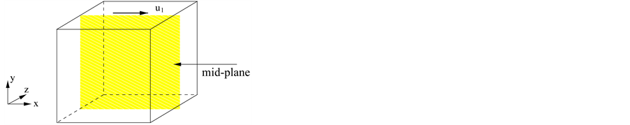
Figure 1. The lid-driven cavity.
expressed in terms of the characteristic length , the characteristic velocity U, and the constant kinematic viscosity
 . The symbol
  denotes the computational domain. The evolution of the system is studied in the time interval
 . The governing Equations (2)-(3) are supplemented with appropriate no-slip boundary conditions for the fluid velocity
 . As the problem is time-dependent, a given divergence-free velocity field is required as initial condition in the internal fluid domain.
2.2. The Differentially Heated Cavity
In this case the geometry is a cube where all walls are fixed. The flow is generated by a temperature difference between the hot left side wall and the cold right side wall. All other walls are insulated. Figure 2 displays the problem set-up and the geometry. The cavity is given in non-dimensional coordinates by  with the origin of the coordinate system located in the lower left corner of the cavity.
With the Boussinesq approximation the fluid is considered as incompressible. The mathematical model includes the advection-diffusion temperature equation. Therefore the buoyancy term in the momentum equations incorporates the influence of the temperature field. The non-dimensional Boussinesq equations read
 (5)
(5)
 (6)
(6)
 (7)
(7)
where T is the temperature, the air Prandtl number  and the Rayleigh number is defined as
 (8)
(8)
with  the gravity,
  the fluid thermal expansion coefficient,
  the temperature difference between the two lateral walls, L the height of the cavity and
  the thermal diffusivity, respectively.
For high Rayleigh numbers of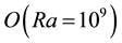 , the flow shows a main convective rotating core with two recirculating pockets located in the corner regions and hook-like structures. These structures present high curvature time-averaged streamlines located between the recirculation pocket and the primary counterflow outside the vertical boundary layer. A full description of these phenomena is given in [10] [13] [16] .
3. The Filtered Boussinesq Equations and LES Models
3.1. Filtered Boussinesq Equations
In this section we present the LES Boussinesq equations to get acquainted with the filtering procedure and the LES modeling. For the LDC case, the LES NS equations are an isothermal subset of the Boussinesq equations as the model does no longer contain the buoyancy term in the momentum equations and the temperature equation.
Filtering the Navier-Stokes and temperature equations, we obtain the filtered Boussinesq equations
 (9)
(9)
Figure 2. The differentially heated cavity.
 (10)
(10)
 (11)
(11)
with the subgrid scale (SGS) tensor 
 (12)
(12)
and the subgrid scale heat flux:
 (13)
(13)
The filtered variables denoted by an overbar are computed as a convolution with a filter kernel G. If we filter the variable  we have
 (14)
(14)
The filters will be presented in section 4.2.
3.2. Subgrid-Scale Field and Reynolds Decomposition
By the filtering operation (14), any variable is decomposed into a resolved part  and the subgrid-scale field
 (15)
(15)
The decomposition of a statistically stationary flow field  in its ensemble average
  and a fluctuating part
  is known as the Reynolds decomposition.
In a LES, in general only the filtered flow solution  is known but not the subgrid-scale field
 . We define the notation
  for the fluctuating part of a filtered field
 (16)
(16)
In the following, we assume that the turbulent flow has reached a statistically steady state, and the Reynolds average is computed as a time average
 (17)
(17)
3.3. LES Models
The additional variables  and
and  in Equations (12)-(13) need to be modeled.
3.3.1. Dynamic Smagorinsky Model
The subgrid scale tensor uses the dynamic Smagorinsky model [5] [6]
 (18)
(18)
where the SGS viscosity is computed by the relation
 (19)
(19)
Here the quantity  is related to the mesh size. The reader is referred to [10] for a detailed description of the filter width in the SEM framework.
The subgrid heat flux is modelled by a subgrid diffusivity
 (20)
(20)
where the SGS diffusivity is evaluated as
 (21)
(21)
and is based on a Reynolds analogy assumption.
The Smagorinsky constant  in Equation (19) and the subgrid Prandtl number
  in (21) will be cal-
culated with the help of the dynamic procedure that uses a coarser test filter denoted by . Usually the ratio of the length-scale
  associated with the test-filter and the grid length-scale
  is chosen as two (cfr. [10] ). The
process allows for the adaption of these parameters to the characteristics of the local flow. The assumption behind this approach rests on a scale-similarity hypothesis which considers that the behavior of the smallest resolved scales is similar to the modeled subgrid scales. The application of the test filter to the filtered Boussinesq equations produces twice filtered equations. The Germano identities allow the evaluation of the difference between the residual stress tensor and the residual heat flux resulting from the double-filtered quantities, namely , and the filtered subgrid scale variables, i.e.


We note that  and
and  are composed of explicit terms that are readily computed. The subgrid heat flux models for once and twice filtered temperature equation are defined by the relationships

3.3.2. Approximate Deconvolution Method
The approximate deconvolution method (ADM) defilters the filtered fields. Following the lead of Stolz et al. [17] [18] , we suppose that the inverse of G in Equation (14) exists and can be evaluated through a finite series in . Therefore the velocity field resulting from the ADM is written as
 (22)
(22)
where  is an approximation of the exact inverse
 . An explicit series approximation is due to van Cittert
 (23)
(23)
where I is the identity operator.
Typical deconvolutions to third or fifth order are given by

 (24)
(24)
with the notation  indicating that the velocity field is filtered k times.
The subgrid scale tensor is computed as
 (25)
(25)
3.3.3. ADM-DMS Model
Because the approximate deconvolution method does not take account of interactions from the computational grid unresolved scales, it needs to be supplemented with a dissipative term. Stolz et al. used an empirical relaxation term to stabilize the computation. Another possibility is to combine the ADM model with a subgrid- viscosity model. The subgrid scale tensor is modeled by the relation
 (26)
(26)
The ADM-DMS was introduced by Bouffanais in his thesis [19] and in Habisreutinger et al. [15] . The mixed scale (MS) model computes a weighted geometric average of the models based on the large scales and those based on the energy at the cutoff, denoted by , as proposed by Loc and Sagaut [3] . In [15] the ADM was coupled with the full MS model leading to the equation
 (27)
(27)
 (28)
(28)
 (29)
(29)
The ADM-DMS method with  was applied to the DHC in [20] .
4. Spectral Element Method
4.1. Space and Time Discretizations
The spectral element method (SEM) decomposes the computational domain into  macro-elements where
  denotes the number of elements in the i-th direction. The space discretization of the velocity
  and temperature T fields is performed using Lagrange-Legendre approximation polynomials defined on a Gauss- Lobatto-Legendre (GLL) grid, built as a tensor product of one-dimensional grid points that are the roots of the relation
 (30)
(30)
where  is the Legendre polynomial of degree N and
  is the reference or parent element.
In order to avoid spurious pressure modes, the pressure p is staggered and approximated on a Gauss-Legendre (GL) grid based on points that are the roots of the equation
 (31)
(31)
From the functional point of view velocity and pressure are in  spaces of polynomial degree N and
 , respectively.
The discrete equations are designed using the weak formulation of the Galerkin method. The continuous integrals of the weak formulation are approximated by Gauss-Legendre numerical quadratures. With the notations borrowed from the monograph [4] , the semi-discrete problem corresponding to the Boussinesq equations (9)-(11) generates a set of non-linear algebraic-differential equations
 (32)
(32)
 (33)
(33)
 (34)
(34)
where  is the diagonal mass matrix,
  the stiffness matrix,
  the discrete gradient,
  the non- linear convection operator and
  the discrete divergence (transpose of
 ). The source term
  includes the subgrid tensor and the buoyancy term, while
  contains the subgrid heat flux.
The time integration scheme rests upon an implicit treatment of the transient Stokes operator and the linear diffusive terms in order to avoid the stringent stability restrictions. This is performed by an Euler backward scheme of order two (Euler2). The non-linear terms are treated explicitly by extrapolation in time (EXT2). The global scheme Euler2/EXT2 has no splitting error and is globally of second order accuracy. A real advantage of SEM comes from the minimal numerical dissipation and dispersion. However the explicit treatment of the advection term imposes a  condition on the time step

The spectral element method is implemented in the toolbox Speculoos [21] that is available as an open source software in [22] .
4.2. Filtering
Two types of filters may be used in the SEM methodology.
4.2.1. Nodal Filtering
The nodal filter due to Fischer and Mullen [8] acts in physical space. Introducing  the set of Lagrange-Legendre interpolant polynomials of degree N based on the GLL grid nodes
 , the rectangular interpolation matrix operator
  of size
  is such that
 (35)
(35)
Therefore, the matrix operator of order M
 (36)
(36)
interpolates on the GLL grid of degree M a function defined on the GLL grid of degree N and transfers the data back to the original grid. This process eliminates the highest modes of the polynomial representation. A one- dimensional representation of the filter is given by the relation
 (37)
(37)
with . In all calculations reported in the sequel,
 .
.
4.2.2. Modal Filter
Here the variable is filtered in the spectral Legendre space that is built on the hierarchical basis (cf. [7] )

In the spectral space a low-pass filter is easily implemented and allows to prune the high-wave number spurious modes. A fully detailed description is yielded in [10] .
For the ADM-DMS model, the modal filter was used on a polynomial space of degree 8. Figure 3 shows the transfer function that was used by Habisreutinger et al. [15] . When the filter is applied to a flow field, every mode determined from the polynomial basis is multiplied by the corresponding value of the transfer function. Because the filter transfer function is nowhere zero and due to the finite dimensional polynomial space, it is possible to compute an exact filter inverse. This exact filter inverse and the approximate deconvolutions of third and fifth order are also shown in Figure 3. We note that the approximate deconvolution of fifth order is very close to the exact filter inverse.
5. Under-Resolved DNS of the Lid-Driven Cavity Problem
The ADM-DMS model was first applied to the lid-driven cavity problem as reported in [15] . LES simulations of the same problem with the dynamic Smagorinsky model and a mixed model proposed by Zang et al. [23] can be found in reference [14] . Here, we perform an under-resolved DNS (UDNS) of the lid-driven cavity problem. The spectral element resolution is the same as in the LES computations of Bouffanais, but no model is used. A detailed description of this flow problem is given in [12] [14] . Table 1 presents the values of the numerical parameters for the DNS and UDNS calculations.
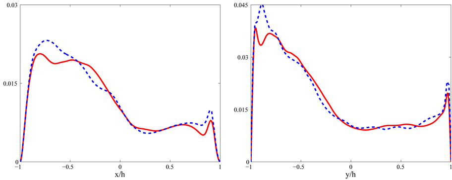
For a quantitative comparison between the UDNS and the DNS, we plot first-order statistics in the mid-plane , namely
  on the vertical centerline
  and
and  on the horizontal centerline
  in Figure 4. These are the same statistics given in the references [14] [15] [19] . The mean fields along the center- lines of the UDNS shown in Figure 4 virtually match the DNS solution.
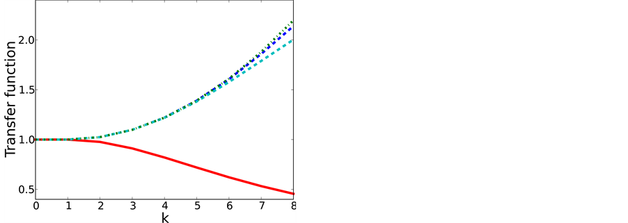
Figure 3. Transfer function of filter (red, solid line), approximate deconvolution of fifth order (blue, dashed line), approximate deconvolution of third order (cyan dashed line) and exact filter inverse (green, dash-dotted line).

Table 1. Numerical parameters of DNS and UDNS computations for the lid-driven cavity.
 (a) (b)
Figure 4. In the mid-plane , DNS (red, solid line) and UDNS (blue, dashed line). (a)
  on the line
 , (b)
, (b)  on the line
 .
.
Now we plot second-order statistics in the mid-plane  on the vertical centerline
  and on the horizontal centerline
  in Figure 5. In the Figures 5 (a)-(f) three components of the Reynolds stress are shown. The UDNS produces correct second order statistics with only minor differences compared to the DNS. Especially in figures (a), (b) and (e), the UDNS overpredicts the values of the peak and in (d) the value of the peak is underpredicted. Note that for the case (e), the statistical values are of small amplitude
 .
.
The comments made about the transfer function in section 4.2.2 raise the question, if it would be a good idea to use the exact filter inverse to model the subgrid-scale tensor (12). Such a model could be readily implemented. But since no information is lost, the filtering can be considered as a change of variables and according to Domaradzki et al. [24] [25] is fundamentally equivalent to an under-resolved DNS. In view of the new UDNS results presented here, in our opinion it remains an open question if ADM is beneficial with the modal filter and how exactly an ADM-based model should be implemented in this context.
6. Under-Resolved DNS of the Differentially Heated Cavity
In order to better understand the efficiency and performance of the LES models, we carried out two under- resolved direct numerical simulations (UDNS) of the DHC. These simulations used the same computational parameters as the LES simulations published in [10] , but with no model for the subgrid-scale variables. The computational parameters of the UDNS and the DNS are shown in Table 2.
We evaluate the number of grid points for the case UDNS1000 in one direction as the product of the number of elements in one direction times the polynomial degree (The number of grid points in a direction within one element is equal the polynomial degree plus one, but values at the element boundaries need to be counted only once). Therefore, the total number of grid points for the case UDNS1000 is 512,000. For the DNS, the total number of grid points is 4,826,809 or a factor 9.4 larger. The two cases, UDNS512 and UDNS1000, correspond to the two LES computations (cf. [10] ) denoted previously as LES512 and LES1000 with 512 elements and 1000 elements, respectively. The polynomial degree is 8 in both cases. With respect to the finest spectral element mesh, the UDNS1000 represents only 11% of the DNS grid points. Due to the coarse under-resolution, the UDNS512 simulation becomes unstable as spurious energy is built up in the highest Legendre modes. Surprisingly, the case UDNS1000 is not only stable, but the flow statistics are also rather accurate and even more accurate than the LES simulations presented in [10] .
In Figure 6 we show the decomposition of the computational domain in spectral elements. The first element is chosen to cover the thin boundary layers at the walls and the interior elements follow a geometric progression of ratio 1.3. In spanwise direction, the flow is close to be two-dimensional with predominant three-dimensional effects close to the spanwise end walls. The sizes of the interior elements are chosen to be uniform except near
 (a) (b)
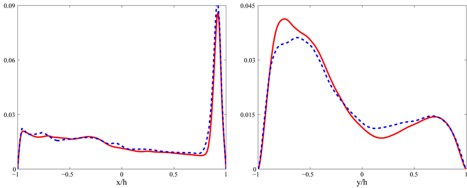 (c) (d)
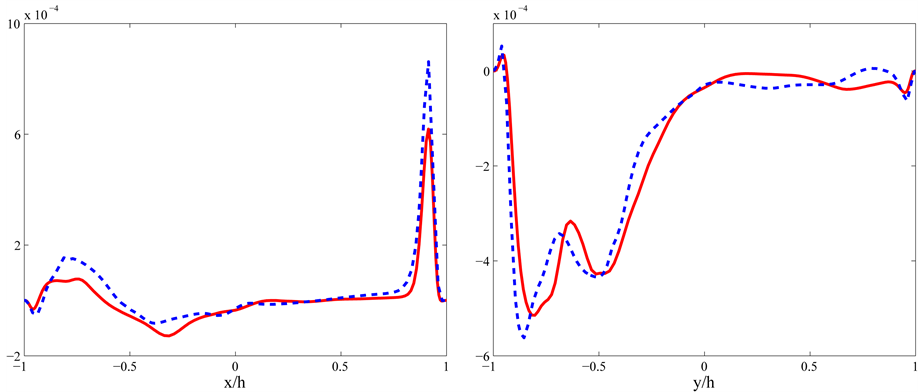 (e) (f)
Figure 5. In the mid-plane , DNS (red, solid line) and UDNS (blue, dashed line). (a)
  on the line
 , (b)
, (b)  on the line
 , … figure continued on page 12.
 (a) (b)
Figure 6. Spectral element decomposition with 10 × 10 × 10 elements. (a) View in any plane normal to y, (b) view in any plane normal to x or z.
Table 2. Numerical parameters of DNS and UDNS simulations for differentially heated cavity.
the walls (cfr. Figure 6(b)). A detailed discussion of the issue on how to choose the spectral element discretization was given in [10] .
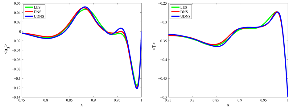
In Figure 7(a) and Figure 7(b), we compare in the mid-plane  the profile of the mean values of the velocity component
  and the temperature
  along the line
 , for DNS in red, UDNS in blue and LES with the dynamic Smagorinsky model with subgrid Prandtl number in green. These profiles cross the turbulent recirculation pocket.
The comparison for the velocity component  in Figure 8 is done in the mid-plane along the line
 . This is selected because for higher z-values the absolute value of this velocity component becomes very small. These are the same flow statistics that were presented for the LES simulations in [4] . The agreement with DNS data is very good and the maximal pointwise error is
  along these lines.
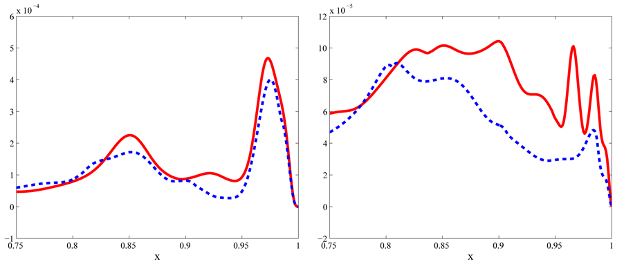
In Figure 9 we show the normal stresses ,
,  ,
,  and the temperature variance
  in the mid-plane
  along the line
 . The normal stresses
 ,
,  and the temperature variance
  are accurately predicted with pointwise maximal errors of
 ,
,  and
and , respectively. For the normal stress
 , the relative difference between DNS and UDNS1000 is higher, but this is only because this normal stress is about one order of magnitude smaller. It is also interesting to note that the accuracy close to the wall is very high, which is a sign that the sudden increase of the spectral element size has no negative impact on the accuracy. Compared to the LES simulations with the dynamic Smagorinsky model and subgrid Prandtl number, we conclude that a UDNS with at least 1000 elements provides the same accuracy.
7. Conclusions
The UDNS was done with a Legendre spectral element code presented in [21] , while the DNS results were produced with a Chebyshev spectral method described in [12] [13] .
Although it is unclear how the accuracy of two different numerical methods can be compared, there is no doubt that the resolution of UDNS1000 is coarser than the one in the DNS. It is not possible to perform a
 (a) (b)
Figure 7. Average  and
and  profiles in the mid-plane
  along the line
 .
.

Figure 8. Average  profile in the mid-plane
  along the line
 . DNS in red, UDNS in blue.
 (a) (b)
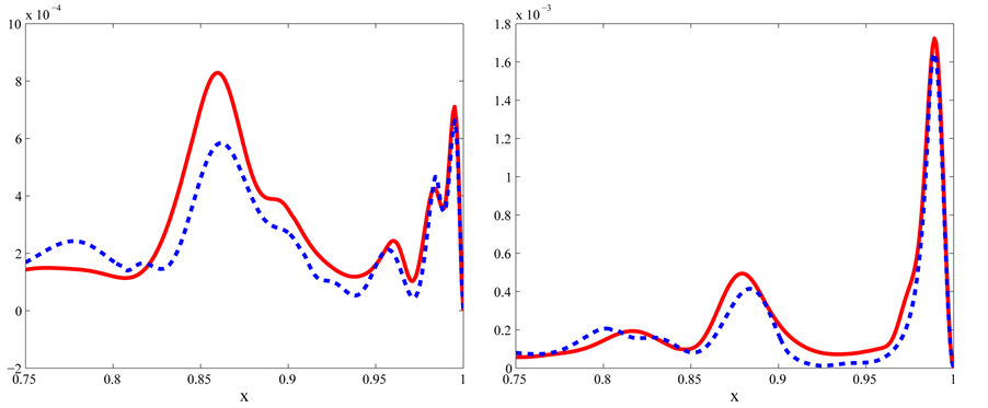 (c) (d)
Figure 9. Comparison of DNS (solid, red line) with UDNS (dashed, blue line) in mid-plane  along the line
 : (a) Normal stress
 , (b) normal stress
 , (c) normal stress
 , (d) temperature variance
 .
.
simulation with significantly less grid points using the Chebyshev spectral program as the computation blows up after a while due to the under-resolution. In our opinion, the high accuracy of the SEM UDNS is linked to the fact that a higher order method with domain decomposition is used. It seems that the Chebyshev spectral method is more sensitive to the under-resolution than the Legendre spectral element method, especially as the grid points scale like  near the walls and as
  in the center of the grid. Furthermore, the Chebyshev collocation method is a global method. Therefore any under-resolution in a part of the domain is affecting the flow solution everywhere. In the spectral element computation, we use a very weak filter of Fischer and Mullen (
 ) [8] , introduced in Section 4.2.1. This weak filtering procedure is implemented to stabilize the spectral element computations to get rid of the spurious energy that builds up in the highest wavenumber modes. One possible explanation for the accurate results of the UDNS is that on a coarse grid and for an under-resolved flow, this stabilizing procedure acts as an implicit LES.
The improvement of the available algorithms should involve more stable time schemes in order to avoid the stringent CFL condition of the explicit treatment of the non-linear terms. That could be achieved by explicit schemes with a larger stability region or by resorting to implicit schemes.
Acknowledgments
This research has been funded by the ARTIST Consortium Project headed by the Paul Scherrer Institute and its support is greatly acknowledged. The LES simulations were carried out on the Pleiades-2 cluster at EPFL-STI- IGM. For the largest simulations the supercomputers Blue Gene/P at EPFL and the Rosa-Cray XT 5 computer at CSCS, Manno, Switzerland were used. The financial support for CADMOS and the Blue Gene/P system is provided by the Canton of Geneva, Canton of Vaud, Hans Wilsdorf Foundation, Louis-Jeantet Foundation, University of Geneva,University of Lausanne, and Ecole Polytechnique Fédérale de Lausanne. This work was supported by a grant from the Swiss National Supercomputing Centre (CSCS) under project ID s328. E. Leriche would like to acknowledge the ERCOFTAC visiting program for several stays at EPFL.
Cite this paper
ChristophBosshard,Michel O.Deville,AbdelouahabDehbi,EmmanuelLeriche, (2015) UDNS or LES, That Is the Question. Open Journal of Fluid Dynamics,05,339-352. doi: 10.4236/ojfd.2015.54034
References
- 1. Berselli, L.C., Iliescu, T. and Layton, W.J. (2006) Mathematics of Large Eddy Simulation of Turbulent Flows. Springer, Berlin.
- 2. Deville, M.O. and Gatski, T.B. (2012) Mathematical Modeling for Complex Fluids and Flows. Springer, Berlin.
http://dx.doi.org/10.1007/978-3-642-25295-2 - 3. Sagaut, P. (2006) Large Eddy Simulation for Incompressible Flows. Springer, Berlin.
- 4. Deville, M.O., Fischer, P.F. and Mund, E.H. (2002) High-Order Methods for Incompressible Fluid Flow. Cambridge University Press, Cambridge.
http://dx.doi.org/10.1017/CBO9780511546792 - 5. Germano, M., Piomelli, U., Moin, P. and Cabot, W.H. (1991) A Dynamic Subgrid-Scale Eddy Viscosity Model. Physics of Fluids A: Fluid Dynamics, 3, 1760-1765.
http://dx.doi.org/10.1063/1.857955 - 6. Lilly, D.K. (1992) A Proposed Modification of the Germano Subgrid-Scale Closure Method. Physics of Fluids A: Fluid Dynamics, 4, 633-635.
http://dx.doi.org/10.1063/1.858280 - 7. Boyd, J.P. (1998) Two Comments on Filtering for Chebyshev and Legendre Spectral and Spectral Element Methods. Journal of Computational Physics, 143, 283-288.
http://dx.doi.org/10.1006/jcph.1998.5961 - 8. Fischer, P.F. and Mullen, J. (2001) Filter-Based Stabilization of Spectral Element Methods. Comptes Rendus de l’Académie des Sciences, Series I, Mathematics, 332, 265-270.
http://dx.doi.org/10.1016/S0764-4442(00)01763-8 - 9. Blackburn, H.M. and Schmidt, S. (2003) Spectral Element Filtering Techniques for Large Eddy Simulation with Dynamic Estimation. Journal of Computational Physics, 186, 610-629.
http://dx.doi.org/10.1016/S0021-9991(03)00088-3 - 10. Bosshard, C., Dehbi, A., Deville, M., Leriche, E., Puragliesi, R. and Soldati, A. (2013) Large Eddy Simulation of the Differentially Heated Cubic Cavity Flow by the Spectral Element Method. Computers & Fluids, 86, 210-227.
http://dx.doi.org/10.1016/j.compfluid.2013.07.007 - 11. Leriche, E. (2006) Direct Numerical Simulation of Lid Driven Cavity at High Reynolds Numbers. Journal of Scientific Computing, 27, 335-345.
http://dx.doi.org/10.1007/s10915-005-9032-1 - 12. Leriche, E. and Gavrilakis, S. (2000) Direct Numerical Simulation of the Flow in a Lid-Driven Cubical Cavity. Physics of Fluids, 12, 1363-1376.
http://dx.doi.org/10.1063/1.870387 - 13. Puragliesi, R. (2010) Numerical Investigation of Particle-Laden Thermally Driven Turbulent Flows in Enclosure. PhD Thesis, No. 4600, EPF Lausanne, écublens.
- 14. Bouffanais, R., Deville, M.O. and Leriche, E. (2007) Large-Eddy Simulation of the Flow in a Lid-Driven Cubical Cavity. Physics of Fluids, 19, Article ID: 055108.
http://dx.doi.org/10.1063/1.2723153 - 15. Habisreutinger, M.A., Bouffanais, R., Leriche, E. and Deville, M.O. (2007) A Coupled Approximate Deconvolution and Dynamic Mixed Scale Model for Large-Eddy Simulation. Journal of Computational Physics, 224, 241-266.
http://dx.doi.org/10.1016/j.jcp.2007.02.010 - 16. Puragliesi, R., Dehbi, A., Leriche, E., Soldati, A. and Deville, M.O. (2011) DNS of Buoyancy-Driven Flows and Lagrangian Particle Tracking in a Square Cavity at High Rayleigh Numbers. International Journal of Heat and Fluid Flow, 32, 915-931.
http://dx.doi.org/10.1016/j.ijheatfluidflow.2011.06.007 - 17. Stolz, S. and Adams, N.A. (1999) An Approximate Deconvolution Procedure for Large-Eddy Simulation. Physics of Fluids, 11, 1699-1701.
http://dx.doi.org/10.1063/1.869867 - 18. Stolz, S., Adams, N.A. and Kleiser, L. (2001) An Approximate Deconvolution Model for Large-Eddy Simulation with Application to Incompressible Wall-Bounded Flows. Physics of Fluids, 13, 997-1015.
http://dx.doi.org/10.1063/1.1350896 - 19. Bouffanais, R. (2007) Simulation of shear-driven flows: transition with a free surface and confined turbulence. PhD Thesis, No. 3837, EPF Lausanne, écublens.
- 20. Bosshard, C. (2012) Large Eddy Simulation of Particle Dynamics inside a Differentially Heated Cavity. PhD Thesis, No. 5297, EPF Lausanne, écublens.
- 21. Dubois-Pèlerin, Y., Van Kemenade, V. and Deville, M.O. (1999) An Object-Oriented Toolbox for Spectral Element Analysis. Journal of Scientific Computing, 14, 1-29.
http://dx.doi.org/10.1023/A:1025677921253 - 22. Speculoos. Spectral Element Analysis Software for the Numerical Solution of Partial Differential Equations; 1998- 2013.
http://sourceforge.net/projects/openspeculoos/ - 23. Zang, Y., Street, R.L. and Koseff, J.R. (1993) A Dynamic Mixed Subgrid-Scale Model and Its Application to Turbulent Recirculating Flows. Physics of Fluids A: Fluid Dynamics, 5, 3186-3196.
http://dx.doi.org/10.1063/1.858675 - 24. Domaradzki, J.A. and Adams, N.A. (2002) Direct Modelling of Subgrid Scales of Turbulence in Large Eddy Simulations. Journal of Turbulence, 3, 024.
http://dx.doi.org/10.1088/1468-5248/3/1/024 - 25. Domaradzki, J.A., Loh, K.C. and Yee, P.P. (2002) Large Eddy Simulations Using the Subgrid-Scale Estimation Model and Truncated Navier-Stokes Dynamics. Theoretical and Computational Fluid Dynamics, 15, 421-450.
http://dx.doi.org/10.1007/s00162-002-0056-y