Open Journal of Fluid Dynamics
Vol.3 No.2(2013), Article ID:32662,11 pages DOI:10.4236/ojfd.2013.32009
Non Linear Vortex Structures in Stratified Fluid Driven by Small-Scale Helical Force
1Université de Toulouse [UPS], CNRS, Institut de Recherche en Astrophysique et Planétologie, Toulouse Cedex, France
2Institute for Single Cristals, Nat. Academy of Science Ukraine, Kharkov, Ukraine
Email: anatoly.tour@irap.omp.eu, *yanovsky@isc.kharkov.ua
Copyright © 2013 Anatoly Tur, Vladimir Yanovsky. This is an open access article distributed under the Creative Commons Attribution License, which permits unrestricted use, distribution, and reproduction in any medium, provided the original work is properly cited.
Received April 8, 2013; revised May 8, 2013; accepted May 16, 2013
Keywords: Vortex Structures; Large Scale Instability; Small Scale Helical Force; AKA-Effect
ABSTRACT
In this work we consider the effect of a small-scale helical driving force on fluid with a stable temperature gradient with Reynolds number . At first glance, this system does not have any instability. However, we show that a large scale vortex instability appears in the fluid despite its stable stratification. In a non-linear mode this instability becomes saturated and gives a large number of stationary spiral vortex structures. Among these structures there is a stationary helical soliton and a kink of the new type. The theory is built on the rigorous asymptotical method of multi-scale development.
1. Introduction
The importance of the generation processes of large-scale coherent vortex structures in hydrodynamics is well known. A large-scale vortex means a vortex which is generated by a much smaller scale force or in turbulence with a characteristic scale much smaller than a vortex scale. When these coherent structures appear in smallscale turbulence they play a key role in transfer processes (see for instance [1]). Numerical and laboratory experiments [2-7], confirm the existence of coherent vortex structures, especially for two-dimensional or quasi twodimensional turbulence [7-9]. Notably, they are well observed in geophysical hydrodynamics like various cyclones in the planet’s atmospheres [10,11]. Sometimes the appearance of large scale vortex structures is accompanied by the inverse cascade of energy both in the three-dimensional case (AKA-effect [12]), and in quasitwo-dimensional cases as well [3-6,8,9]. It may be said that the inverse cascade itself is also one of the mechanisms of the generation of large-scale structures [4,13]. The generation of large scale slow movements by small scale external forces in a rotating stratified fluid was also studied numerically in works [14,15]. One of the important large scale instabilities in non compressible fluid is the AKA-effect (Anisotropic Kinetic Alpha effect) which was found in work of Frisch, She and Sulem [16]. In this work a large scale instability appears under the impact of small scale force in which parity is broken (with zero helicity). In the following work [17] the inverse cascade of energy and the non linear mode of instability saturation were studied. Despite the fact that the broken parity is a more general notion than helicity, it is the helicity  which is the widespread mechanism of broken parity in hydrodynamical flow. For instance, the turbulence becomes helical when rotation and stratification are taken into account [18-20]. Therefore one may consider the small-scale helical force the parametrization of this turbulence. The injection of a helical external force into hydrodynamic systems was considered in many works ([21-24]), and as a result it was understood that a small-scale turbulence able to generate large-scale perturbations cannot be simply homogeneous, isotropic and helical [25], but must have additional special properties. In some cases the existence of large-scale instability was shown (vortex dynamo or hydrodynamic
  -effect). (In the magneto hydrodynamics of conductive fluid the
  -effect is well known [26] ). In particular, in work [22] it is shown that large-scale instability exists in convective systems with small-scale helical turbulence. These works as well as the results of numerical modelling are described in detail in review [27], which are focused essentially on the possible application of these results to the issue of tropical cyclone origination.
In this work we consider the theory of large scale vortex generation in stratified fluid under the impact of small scale helical force. Let us suppose that there is a stable temperature stratification in fluid. To this fluid with the Reynolds number  let us apply a smallscale, helical, external force. This force will maintain in the fluid small-scale helical fluctuations of velocity field
  We consider the fluid as being boundless. At first glance there are no instabilities at all in this system. However, we show in this work that despite stable stratification, a large-scale vortex instability appears in the fluid which leads to the generation of large-scale vortex structures. The theory of this instability is built rigourously using the method of asymptotical multi-scale development similar to what was done in work of Frisch, She and Sulem for the theory of AKA-effect [16]. But the equations which we solve differ considerably from equations in work [16]. In addition to linear theory, we also develop and study in details the non-linear theory of this instability saturation. We devote special attention to stationary, non-linear, periodical vortex structures which appear as a result of the saturation of found instability. Among these structures there is a spiral vortex soliton and kink of the new type. In order to distinguish our instability from others in stratified fluid we consider the case of stable stratification. Nevertheless our theory permits the examination of unstable stratification as well by means of substitution
  However, in this case we have to consider that the usual convective instability is eliminated and the Raleigh number is reasonably small.
Our work is arranged as follows: in Section 2 we set forth the formulation of the problem and equations for stable stratification in Boussinesq approximation; in Section 3 we examine the principal scheme of multi scale development and we give secular equations. In Section 4 we describe external force properties and calculate the Reinolds stress. In Section 5 we discuss the non-linear stage of the instability and its saturation. We study the equations of non-linear instability and its stationary solutions. It is shown that due to the hamiltonian nature of these equations a large number of stationary vortex structures of spiral type appear. We also demonstrate that there are solutions in the form of the spiral soliton and the kink of new type. The obtained results are discussed in the conclusion in Section 6.
2. Main Equations and Formulation of the Problem
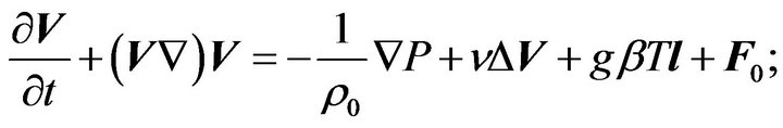
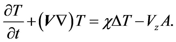
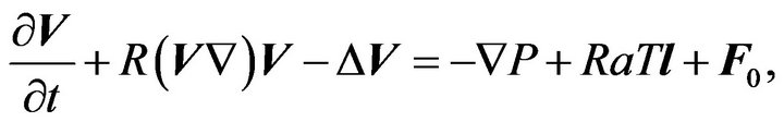
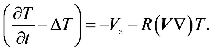
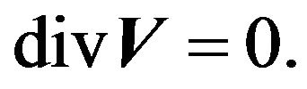
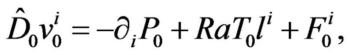
Let us consider the equations for the motion of non compressible fluid with a constant temperature gradient in the Boussinesq approximation:
 (1)
(1)
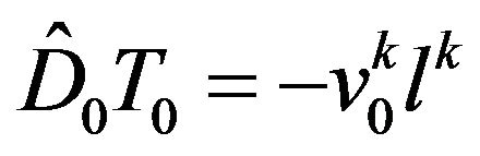
 (2)
(2)
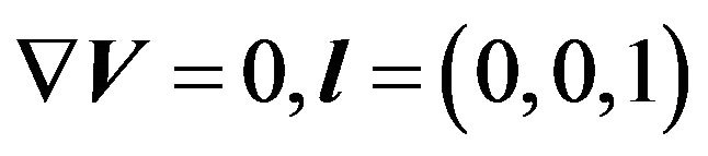 —is the unit vector in the direction of axis
 ,
, —is the thermal expansion coefficient,
 —constant equilibrium gradient of temperature,
 .
.  The buoyancy force and the external force
 are taken into account in Euler Equation (1). Let us note the force
 in the form:
 , where
 —charac teristic scale,
 —characteristic time,
 —characteristic amplitude of external force. We designate characteristic velocity, which is engendered by external force as
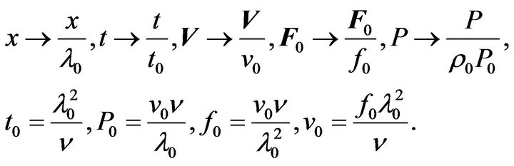
 . We choose the dimensionless variables
 :
:
Then:
where —Reynolds number on the scale
 ,
, —is Prandtl number. We introduce the dimensionless temperature
 , and obtain the equations system:
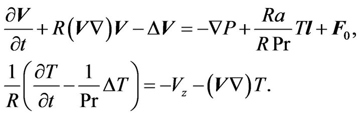
Here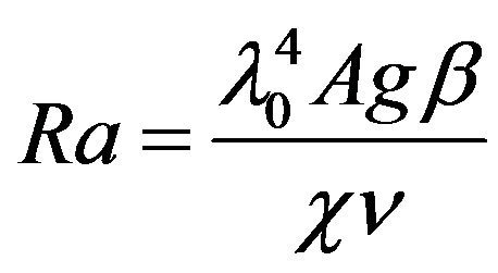 —is Rayleigh number on the scale
 . Further for the purpose of simplification we will consider the case
 . We pass to the new temperature
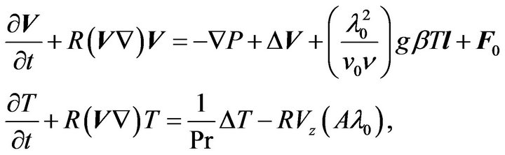
 , and obtain:
 (3)
(3)
 (4)
(4)
Although we essentially pay attention to stable temperature stratification, unstable stratification can also be considered in the frame of this scheme. We use dimensionless writing of the equation more typically for the problem of convection.
We will consider as a small parameter of asymptotical development the Reynolds number 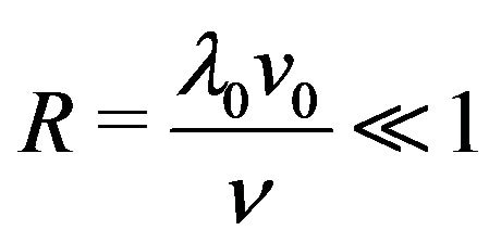 on the scale
 . The parameter
  will be considered neither big nor small, without any impact on development scheme (i.e. outside of the scheme parameters).
Let us examine the following formulation of the problem. We consider the external force as being small and of high frequency. This force leads to small scale fluctuations in velocity and temperature against a background of equilibrium. After averaging, these quickly oscillating fluctuations vanish. Nevertheless, due to small non-linear interactions in some orders of perturbation theory, non zero terms can occur after averaging. This means that they are not oscillatory, that is to say large scale. From a formal point of view these terms are secular, i.e. create conditions for the solvability of the large scale asymptotic development. So, to find and study the solvability equations i.e. the equations for large scale perturbations is actually the purpose of this work. Let us designate further the small scale variables as
 , and large scale ones as
 . The derivative
  is designated
 , the derivative
  is designated
 , and derivatives of large scale variables are
  and
and  respectively (No confusion misunderstanding occurs between the temperature and the large scale time since time is argument and temperature is function). To construct a multi scale asymptotic development we follow the method which is proposed in work [16]. We could start by establishing linear theory for instability development and after that pass to non linear theory, but as the non linear theory is technically less bulky, so we construct the non linear theory directly and then consider the linear limit.
3. The Multi-Scale Asymptotical Development
Let us search the solution for Equations (3) and (4) in the following form:
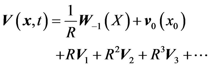 (5)
(5)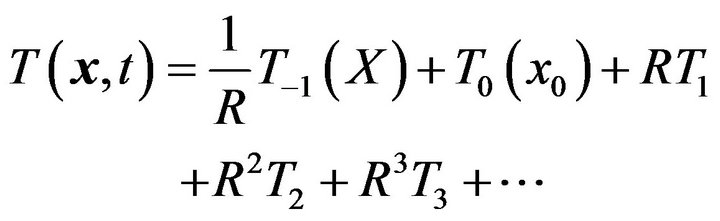 (6)
(6)
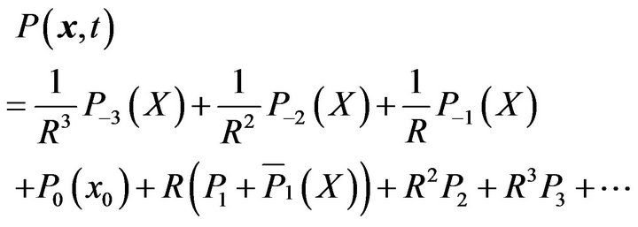 (7)
(7)
First of all, we develop space and time derivatives in Equations (3) and (4) into asymptotical series of the form:
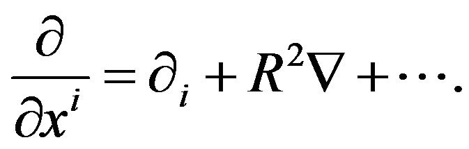 (8)
(8)
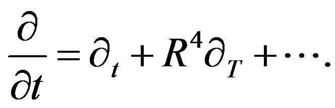 (9)
(9)
Substituting these expressions into the initial Equations (3) and (4) and gathering together the terms of the same order, we obtain the equations of multi scale asymptotical development and write down the obtained equations up to order  inclusive. Let us present the algebraical structure of the asymptotical development of the Equations (3) and (4) for the non linear theory (we will not write indices because they can be restored trivially at any moment). In the order
  there is only the equation:
 (10)
(10)
In the order  we have the equation :
 (11)
(11)
In the order  we get a system of equations:
 (12)
(12)
 (13)
(13)
The system of Equations (12) and (13) gives secular terms:
 (14)
(14)
 (15)
(15)
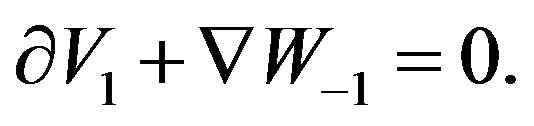
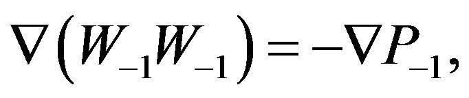
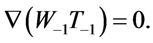
In zero order  we have the following system of equations:
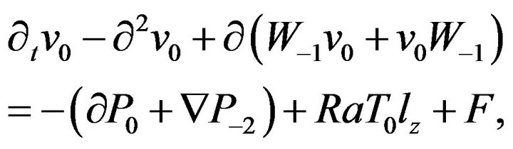 (16)
(16)
 (17)
(17)
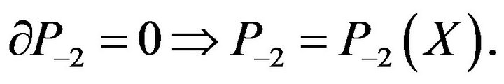
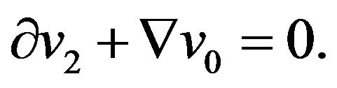
These equations give one secular equation:
 (18)
(18)
Consider the equations of the first approximation R:
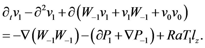 (19)
(19)
 (20)
(20)
 (21)
(21)
From this system of equations follow the secular equations:
 (22)
(22)
 (23)
(23)
 (24)
(24)
The secular Equations (22)-(24), are clearly obviously satisfied for velocity field geometry:
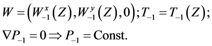 (25)
(25)
In the second order , we obtain equations:
 (26)
(26)
 (27)
(27)
 (28)
(28)
It is easy to see that in the order  there are no secular terms.
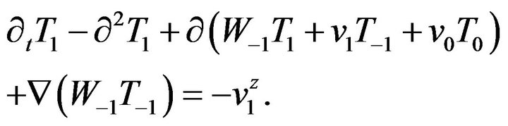
Let us come now to the most important order . In this order we obtain equations:
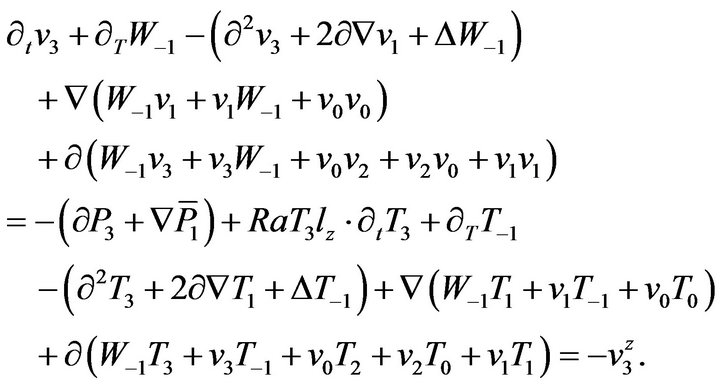 (29)
(29)
 (30)
(30)
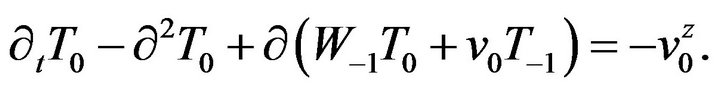
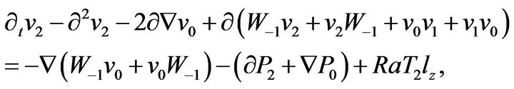
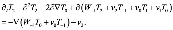
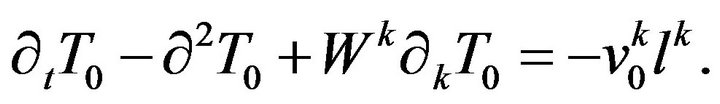
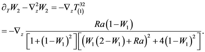
From this we get the main secular equation:
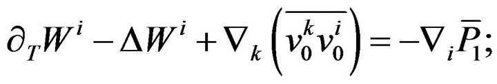 (31)
(31)
 (32)
(32)
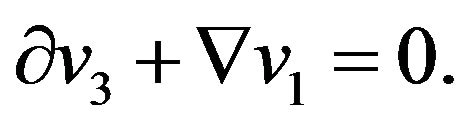
In these equations we do not write the law index . Besides there are secular equations:
 (33)
(33)
 (34)
(34)
 (35)
(35)
The Equations (33)-(35) are satisfied in the previous geometry:
 (36)
(36)
There is also an equation to find the pressure :
:
 (37)
(37)
These formulae show that when one knows the velocity it is possible to restore temperature and pressure.
4. Calculations of the Reynolds Stresses
It is clear that the essential equation for finding the non linear alpha-effect is Equation (31). In order to obtain these equations in the closed form we need to calculate the Reynolds stresses . First of all we have to calculate the fields of zero approximation
  from the asymptotical development in zero order we have the equations:
 (38)
(38)
 (39)
(39)
Let us introduce the operator :
:
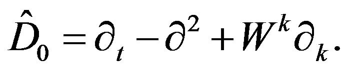 (40)
(40)
Using the operator , we write down Equations (38) and (39) in the form:
 (41)
(41)
 (42)
(42)
Eliminating the temperature and pressure from Equation (41) we obtain:
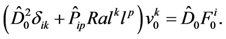 (43)
(43)
Here  is the projection operator:

Dividing this equation by , we can write it in the form:
 (44)
(44)
where  is the operator:
 (45)
(45)
It is easy to make sure by a direct check that the inverse operator  has the form:
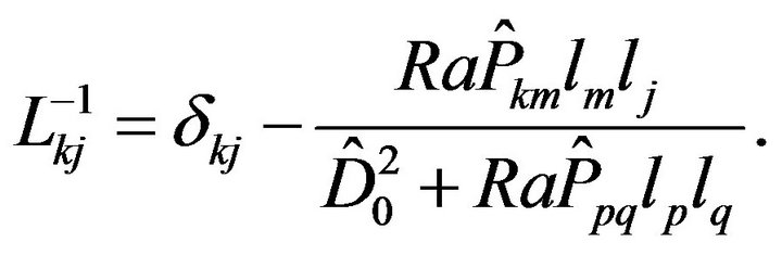 (46)
(46)
 (47)
(47)
Consequently the expression for the velocity and temperature ,
,  takes the form:
 (48)
(48)
 (49)
(49)
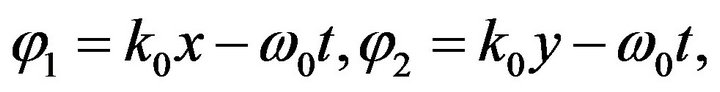
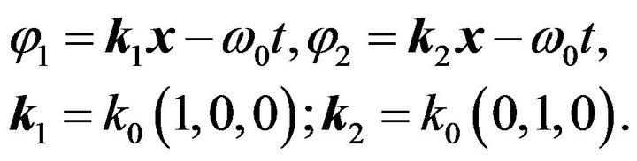
In order to use these formulae we have to specify in explicit form the helical external force . The most simple and natural way is to specify the external force as deterministic. (Certainly, it is possible to specify the external force in a statistical way with specifying random field correlators, but this leads to more bulky calculations). As it is known helicity means that
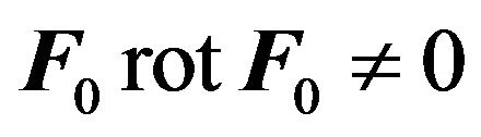 . Let us specify the force
  like so:
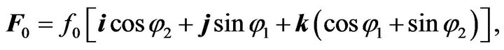 (50)
(50)
where
 (51)
(51)
or
 (52)
(52)
It is evident that , where
 —is the single pseudo scalar, i.e. helicity is equal to:
 (53)
(53)
The formulae (50) and (52) allow us to easily make intermediate calculations, but in the final formulae we obviously shall take  as equal to one, since external force is dimensionless and depends only on dimensionless space and time arguments. The force (50) is physically simple and can be realized in laboratory experiments and in numerical simulation.
It is easy to write down the force (50) in complex form. It is evident that:
 (54)
(54)
where vectors  and
and  has the form:
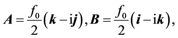 (55)
(55)
and  are given by formulae (52). The effect of the operator
  on proper function
  has obviously the form:
 , where
 is:
is:
 (56)
(56)
From this it is evident that:
 (57)
(57)
 (58)
(58)
 (59)
(59)
 (60)
(60)
From the formulae (48) and (54), follows that the field  is composed of four terms:
  where
where
 (61)
(61)
 (62)
(62)
As was stated earlier, in scalar operators  one can take
 . Then taking into account that
 , we obtain:
 (63)
(63)
 (64)
(64)
Here we introduced the following notations:  . Taking into consideration these formulae we can write down the velocities
  in the form:
 (65)
(65)
 (66)
(66)
In order to calculate the Reynolds stresses we have first of all to calculate the expression:
 (67)
(67)
Taking into account the formula (65), we obtain:
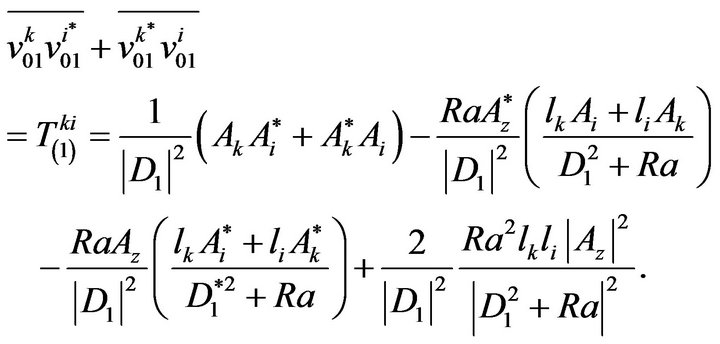 (68)
(68)
Similarly taking into account formula (66), we obtain:
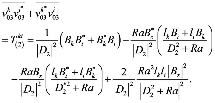 (69)
(69)
It is clear that the components  and
and  are of interest. To begin with we consider the components of the tensor
 .
.
 (70)
(70)
since .
.
 (71)
(71)
The first bracket in the (71) is equal to zero, which is why:
 (72)
(72)
Now consider the component :
:
 (73)
(73)
as far as . Consider now the component
 :
:
 (74)
(74)
The first bracket in the formula (74) is equal to zero, then:
 (75)
(75)
Taking into account:
 (76)
(76)
 (77)
(77)
 (78)
(78)
 (79)
(79)
The components  take the form:
 (80)
(80)
 (81)
(81)
Now, when we have these tensors components, we can obtain closed equations for velocity.
5. Large-Scale Instability and Non Linear Vortex Structures
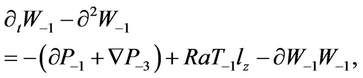
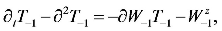
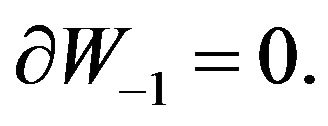
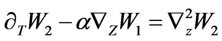
Let us write down in the explicit form the equations for non linear instability:
(82)
(83)
It is easy to see that with small values of the variables  the Equations (82) and (83) are reduced to linear equations and describe the linear stage of instability.
 (84)
(84)
 (85)
(85)
 (86)
(86)
Here  designates the single pseudo scalar because expressions
 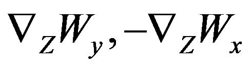 are components of
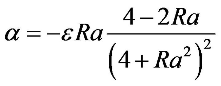
 . The Equations (84) and (85) differ from equation of AKA-effect [16] by the coefficient
  only, but the important difference between our equations and equations of AKA-effect is the presence of the Rayleigh number in
  coefficient. As a result:
  in the non stratified fluid. The Equations (84) and (85) obviously contain an instability which generates large scale vortex structures. Choosing the velocities
  in the form:
 (87)
(87)
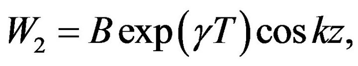 (88)
(88)
we obtain the instability increment 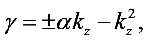 i.e..
i.e..
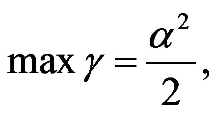 with the
 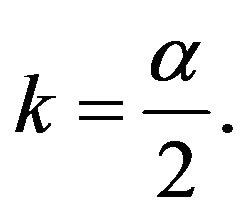 The formulae (87) and
(88) describe a spiral vortex structure (circularly polarized plane wave) with an amplitude which increases exponentially with time. These waves are sometimes called Beltrami runaways since for them there is no usual hydrodynamical interaction . With
  the linear instability vanishes but the non linear remains.
If the external force has a zero helicity, then the  -term vanishes in accordance with the general theorem of Reynolds stress tensor [25]. Helicity is taken into account in the external force structure itself. If the temperature gradient vanishes, then it is evident that the
  -term also vanishes.
It is clear that with the increasing  of the non linear terms decrease and the instability becomes saturated. As a result of the development and stabilization of instability, non linear vortex helical structures appear. The study of the form of these stationary structures is of interest. For that purpose we take (82), (83)
  . Integrating these equations over
 , we obtain:
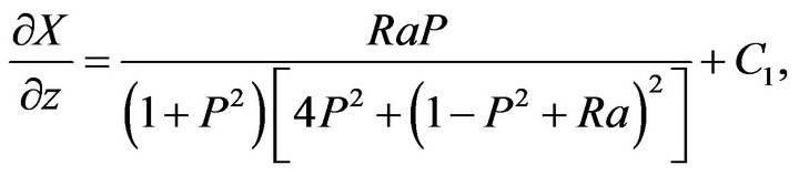 (89)
(89)
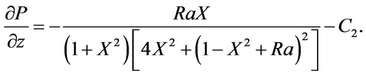 (90)
(90)
Here new variables are introduced 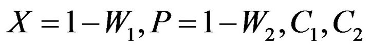 —are integration constants. The system of Equations (89) and (90) can be write down in the hamiltonian form:
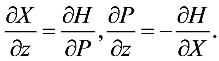 (91)
(91)
Here the variable  plays the role of time and the hamiltonian
  has the form:
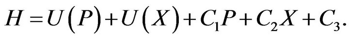 (92)
(92)
where function  has the form:
 (93)
(93)
The function  (92), (93) is obviously the first integral of the equations system (89), (90) and can be found by the direct integration of this system. With
  the function
  is limited above and below as well. That is why the section of this hamiltonian by the constant
 , gives closed periodical trajectories on the phase plane
 , which correspond to the helical vortex structures in real space. Examples of phase pictures for
  and
and  are presented in Figures 1 and 2. (As was already mentioned with
  the instability is essentially non linear). With
  there is only one elliptical point on the phase plane. Closed trajectories correspond to the periodical non linear vortex structures. Despite the fact that
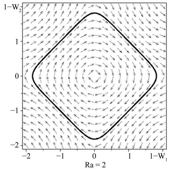
Figure 1. Phase picture of the dynamical system with Ra = 2, C1 = C2 = 0. The bold line shows the phase trajectory which comes out of the point (1,1) and after the “time” Z = L comes back to the same point. This trajectory presents the stationary solution of the boundary problem with the rigid boundaries in the layer whose thickness is L = z.
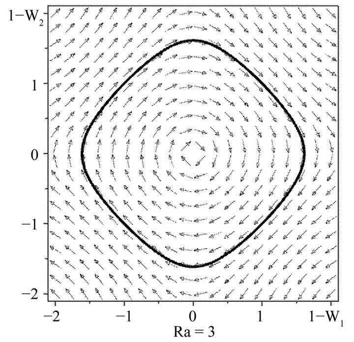
Figure 2. Phase picture of the dynamical system with Ra = 3, C1 = 0, C2 = 0. The bold line shows the trajectory which corresponds to the stationary solution of the boundary problem with rigid boundaries with z = 0 and z = L.
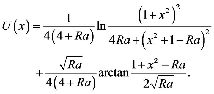
we are mostly interested in a boundless problem, it should be noted that thick closed lines correspond to the non linear structures which are also the solutions of the boundary problem with a rigid boundary:
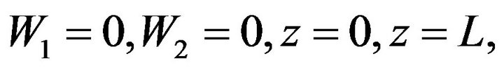
where  is the period over
  phase trajectory, which gets out with
 , from point
  and gets back to the same point with
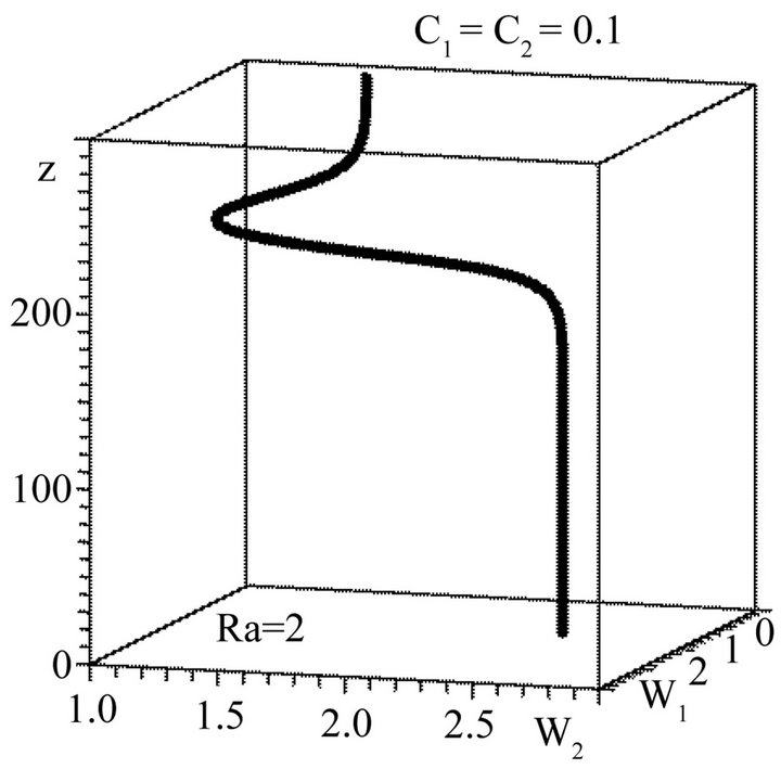
  The space structures of periodical solutions are presented in Figures 3-5. If one of the constants, for instance
 , then one hyperbolic point appears on phase picture. For instance, phase pictures with
  are presented in Figure 6. An example of a periodical nonlinear vortex structure which corresponds to the closed trajectory on a phase plane with
 , is given in Figure 7. In this case the linear instability is obviously absent. The solution which corresponds to the separatrix on Figure 6. is of particular interest. This solution describes the solitary spiral turn of the velocity field around the axe
  (soliton): see Figure 8. Moving away from the soliton the velocity field becomes constant. This kind of soliton was not known earlier. The interesting particularity of this soliton is the fact that it is also the solution for the boundary problem with free boundaries. For this boundary problem [28]:
on the fluid boundary. In addition, boundaries must be at a great distance from soliton, much bigger than the soliton’s characteristic dimensions. In this case at great distances from soliton: . In a case when there are two constants
 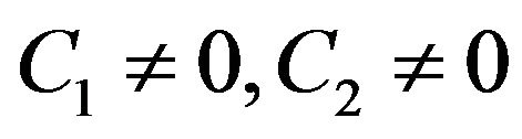 two hyperbolic and two elliptical points appear on the phase picture. The example of this phase picture with C1 = 0.1,
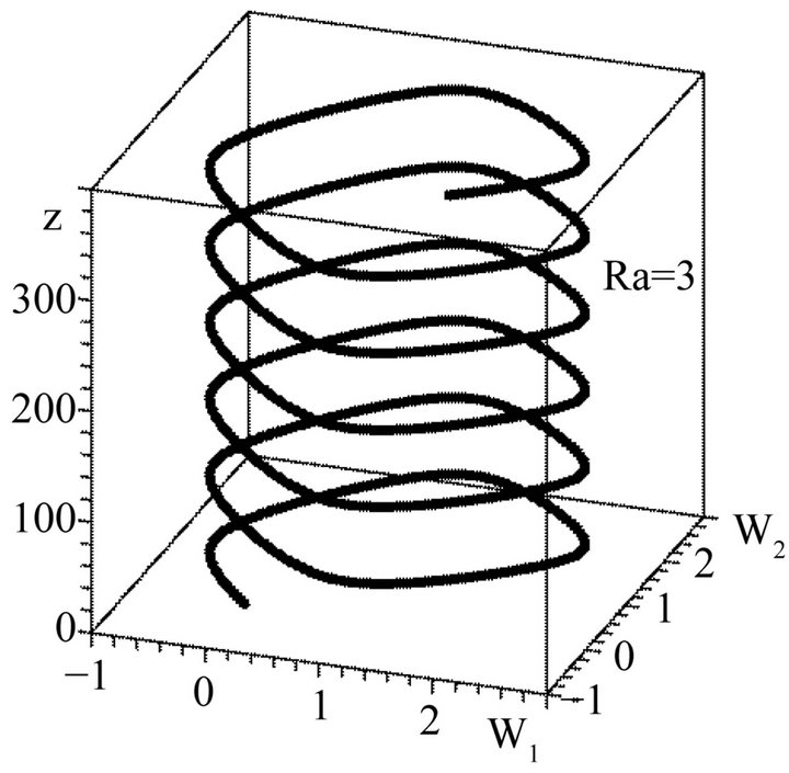
Figure 3. Helical vortex structure with Ra = 3, C1 = 0, C2 = 0.
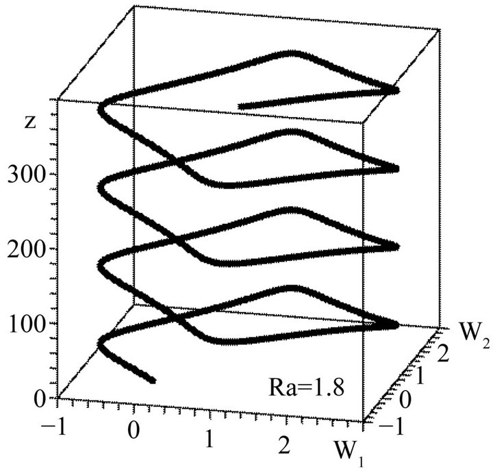
Figure 4. Helical vortex structure with Ra = 1.8, C1 = 0, C2 = 0.
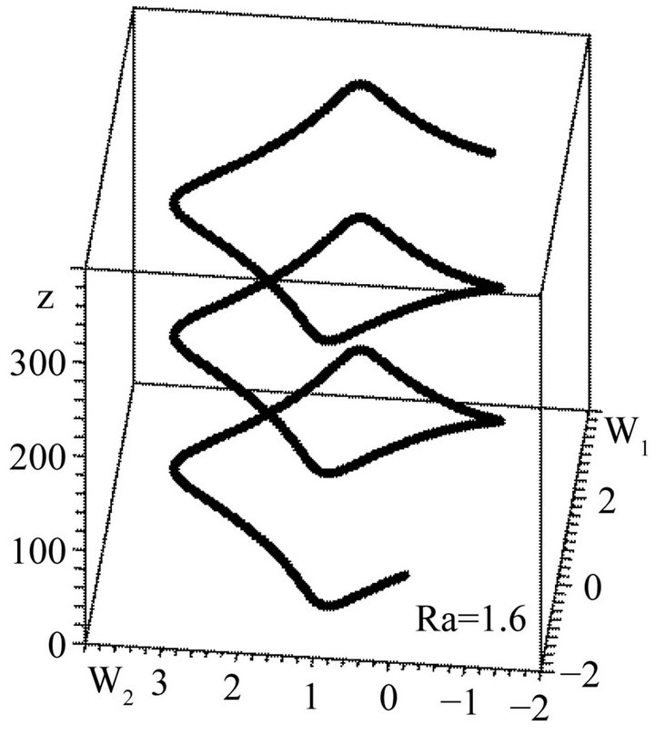
Figure 5. Example of a vortex structure with Ra = 1.6, C1 = 0, C2 = 0.
C2 = 0.1 is shown in Figure 9. As above, the periodic vortex structures correspond to closed trajectories around elliptical points. Localized solutions (solitons) correspond to the separatrix on Figure 9. Since the separatrix connects two different hyperbolic points the soliton has now two different limiting values, with , Figure 10. This soliton is called a kink. Therefore, spiral kinks correspond to the separatrix in Figure 9. These kinks are
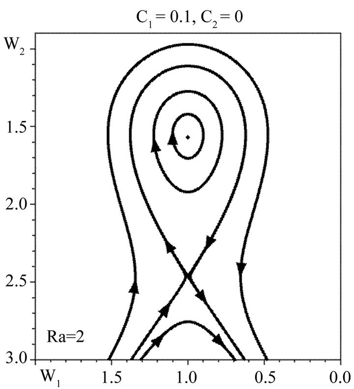
Figure 6. Phase picture of a dynamical system with Ra = 2, C1 = 0, C2 = 0.
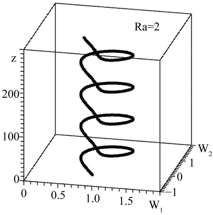
Figure 7. Helical vortex structure with Ra = 2, C1 = 0, C2 = 0. This structure corresponds to the closed trajectory around the elliptical point in Figure 6.
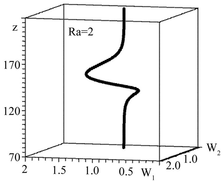
Figure 8. Helical soliton which corresponds to the separatrix in Figure 6 with Ra = 2, C1 = 0, C2 = 0.
also solutions for the boundary problem with free boundaries. Thereby in the hamiltonian scheme which we consider there are three kinds of solutions: periodical waves, solitons and solutions moving to infinity. The last ones are not of interest from the point of view of the problem of large cale instability stabilization. In conclusion it should be remembered that the system of the
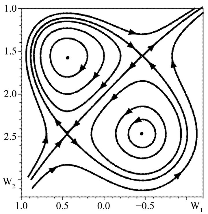
Figure 9. Phase picture of the dynamical system with Ra = 2, C1 = 0.1, C2 = 0.1. One can see the appearance of two hyperbolical and two elliptical points.
Equations (82), (83) is closed. The velocity field  determines the pressure
  and contributes to the equation for temperature (32). Closure of this equation is made in much the same way as closure for velocity. Nevertheless this equation is secondary and here we do not give the result of this closure.
6. Conclusions and Discussion of Results
In this work it is shown that in fluid with stable stratification a large scale instability appears under the action of small scale helical force. The result of the instability is the generation of vortex structures of the Beltrami type. These vortices have the characteristic vertical dimension  and a horizontal dimension much bigger than the vertical one. Since the vertical component of the velocity
  is equal to zero in the main approximation and the stratification is stable, then the found instability does not have any relation to convection. The structure of the equation which describes the instability in linear approximation is the same as the equation of
  -effect or more precisely as the equation of AKA-effect. But as opposed to the AKA-effect,
  is function of Rayleigh number. This means the instability vanishes in the non stratified fluid. As a result instability generates plane spiral waves with circular polarization (Beltrami runaway). With increases in amplitude, the instability and its stabilization are described by non linear theory. With
  the instability has an essentially non linear character from the very beginning. Stationary equations appear to be hamiltonian that is why they are a rich set of periodical spiral vortex structures. Notwithstanding that attention in this work was essentially paid to the boundary free problem, it should be noted that some periodical solutions turn out to be solutions for the boundary problem with rigid boundaries. One of the most interesting to note are the stationary soliton and kink, which correspond to the separatrix on the phase plane. This is a soliton of the new type. In real space it describes one spiral turn of the velocity vector field around the axe z. The soliton and kink are also the solutions for the boundary problem with free boundaries.
Let us return to the formulation of the problem. The external helical force  is given in the explicit form in order to make calculations more transparent. Strictly speaking its explicit form is not very important for the existence of
  -effect itself. It is only necessary that
 . The external force could be chosen statistically with specifying the correlator:
 (94)
(94)
It is fundamental that the last term  (helicity) in this correlator is not equal to zero, otherwise the
  - effect is absent. Nevertheless the statistical method is more bulky since it requires us to specify the functions
  and calculations of rather complicated integrals. If we specify the external force dynamically then averaging over fast oscillations is performed easily. In conclusion it should be noted that temperature stratification is necessary for the existence of the instability. Previously it was supposed that this stratification was stable. However, the formulae for the large scale instability also admit the transition to an unstable fluid stratification, i.e. allow the substitution
  But one has to remember that the number
  has to be sufficiently small so that the usual convective instability should not appear in the system.
REFERENCES
- J. Jimenez, “The Role of Coherent Structures in Modeling Turbulence and Mixing,” Lecture Notes in Physics, Vol. 136, 1981.
- J. C. McWilliams, “The Emergence of Isolated Coherent Vortices in Turbulent Flow,” Journal of Fluid Mechanics, Vol. 146, 1984, pp. 21-43. doi:10.1017/S0022112084001750
- J. Sommeria, “Experimental Study of the Two-Dimensional Inverse Energy Cascade in a Square Box,” Journal of Fluid Mechanics, Vol. 170, 1986, pp. 139-168. doi:10.1017/S0022112086000836
- R. H. Kraichnan, “Inertial Ranges in Two-Dimensional Turbulence,” Physics of Fluids, Vol. 10, No. 7, 1967, pp. 1417-1423. doi:10.1063/1.1762301
- M. Chertkov, C. Connaughton, I. Kolokolov and V. Lebedev, “Dynamics of Energy Condensation in Two-Dimensional Turbulence,” Physical Review Letters, Vol. 99, No. 8, 2007, Article ID: 084501. doi:10.1103/PhysRevLett.99.084501
- D. Byrne, H. Xia and M. Shats, “Robust Inverse Energy Cascade and Turbulence Structure in Three-Dimensional Layers of Fluid,” Physics of Fluids, Vol. 23, No. 9, 2011, Article ID: 095109. doi:10.1063/1.3638620
- Y. Couder and C. Basdevant, “Experimental and Numerical Study of Vortex Couples in Two-Dimensional Flows,” Journal of Fluid Mechanics, Vol. 173, 1986, pp. 225-251. doi:10.1017/S0022112086001155
- J. Paret and P. Tabeling, “Intermittency in the Two-Dimensional Inverse Cascade of Energy: Experimental Observations,” Physics of Fluids, Vol. 10, No. 12, 1998, pp. 3126-3136. doi:10.1063/1.869840
- D. Molenaar, H. J. H. Clercx and G. J. F. van Heijst, “Angular Momentum of forced 2D Turbulence in a Square No-Slip Domain,” Physica D, Vol. 196, No. 3-4, 2004, pp. 329-340. doi:10.1016/j.physd.2004.06.001
- J. Sommeria, S. P. Meyers and H. L. Swinney, “Laboratory Simulation of Jupiter’s Great Red Spot,” Nature, Vol. 331, No. 6158, 1988, pp. 689-693. doi:10.1038/331689a0
- G. Dritschel and B. Legras, “Modeling Oceanic and Atmospheric Vortices,” Physics Today, Vol. 46, No. 3, 1993, pp. 44-51. doi:10.1063/1.881375
- B. Galanti and P. L. Sulem, “Inverse Cascades in ThreeDimensional Anisotropic Flows Lacking Parity Invariance,” Physics of Fluids A, Vol. 3, No. 7, 1991, p. 1778- 1784.
- U. Frisch, “Turbulence: The Legacy of A. N. Kolmogorov,” Cambridge University Press, Cambridge, 1995.
- L. M. Smith and F. Waleffe, “Transfer of Energy to TwoDimensional Large Scales in Forced, Rotating ThreeDimensional Turbulence,” Physics of Fluids, Vol. 11, No. 6, 1999, pp. 1608-1623. doi:10.1063/1.870022
- L. M.Smith and F. Waleffe, “Generation of Slow Large Scales in Forced Rotating Stratified Turbulence,” Journal of Fluid Mechanics, Vol. 451, 2002, pp. 145-168. doi:10.1017/S0022112001006309
- U. Frisch, Z. S. She and P. L. Sulem, “Large-Scale Flow Driven by the Anisotropic Kinetic Alpha Effect,” Physica D, Vol. 28, No. 3, 1987, pp. 382-392. doi:10.1016/0167-2789(87)90026-1
- P. L. Sulem, Z. S. She, H. Scholl and U. Frisch, “Generation of Large-Scale Structures in Three-Dimensional Flow Lacking Parity-Invariance,” Journal of Fluid Mechanics, Vol. 205, 1989, p. 341. doi:10.1017/S0022112089002065
- G. Rudiger, “On the α-Effect for Slow and Fast Rotation,” Astronmische Nachrichten, Vol. 299, No. 4, 1978, pp. 217-222. doi:10.1002/asna.19782990408
- A. Pouquet and P. D. Mininni, “The Interplay between Helicity and Rotation in Turbulence: Implications for Scaling Laws and Small-Scale Dynamics,” Philosophical Transactions of the Royal Society A, Vol. 368, No. 1916, 2010, pp. 1635-1662.
- H. K. Moffatt and A. Tsinober, “Helicity in Laminar and Turbulent Flow,” Annual Reviews of Fluid Mechanics, Vol. 24, 1992, pp. 281-312. doi:10.1146/annurev.fl.24.010192.001433
- S. S. Moiseev, R. Z. Sagdeev, A. V. Tur, G. A. Khomenko and V. V. Yanovsky, “A Theory of Large-Scale Structure Origination in Hydrodynamic Turbulence,” Soviet Physics, Vol. 58, 1983, pp. 1149-1157.
- S. S. Moiseev, P. B. Rutkevich, A. V. Tur and V. V. Yanovsky, “Vortex Dynamos in a Helical Turbulent Convection,” Soviet Physics, Vol. 67, 1988, pp. 263-294.
- E. A. Lupyan, A. A. Mazurov, P. B. Rutkevich and A. V. Tur, “Generation of Large-Scale Vortices through the Action of Spiral Turbulence of a Convective Nature,” Soviet Physics, Vol. 75, 1992, pp. 829-833.
- G. A. Khomenko, S. S. Moiseev and A. V. Tur, “The Hydrodynamic Alpha-Effect in a Compressible Fluid,” Journal of Fluid Mechanics, Vol. 225, No. 1, 1991, p. 355. doi:10.1017/S0022112091002082
- F. Krause and G. Rudiger, “On the Reynolds Stress in Mean Field Hydrodynamics. 1. Incompressible Homogeneous Isotropic Turbulence,” Astronmische Nachrichten, Vol. 295, No. 2, 1974, pp. 93-99. doi:10.1002/asna.19742950205
- H. K. Moffat, “Magnetic Field Generation in Electrically Conducting Fluids,” Cambridge University Press, Cambridge, 1978.
- G. V. Levina, S. S. Moiseev and P. B. Rutkevich, “Hydrodynamic Alpha-Effect in a Convective System,” Advances in Fluid Mechanics, Vol. 25, 2000, pp. 111-162.
- S. Chandrasekhar, “Hydrodynamic and Hydromagnetic Stability,” Dover Publishers, New York, 1961.
NOTES
*Corresponding author.