Journal of Power and Energy Engineering
Vol.04 No.03(2016), Article ID:65224,10 pages
10.4236/jpee.2016.43006
Design of a Fixed-Order Robust Controller to Damp Inter-Area Oscillations in Power Systems
Abdlmnam Abdlrahem1, Parimal Saraf1, Karthikeyan Balasubramaniam1, Ramtain Hadidi1, Alireza Karimi2, Elham Makram1
1Department of Electrical and Computer Engineering, Clemson University, Clemson, USA
2Laboratoired'Automatique, Ecole Polytechnique Fédérale de Lausanne (EPFL), Lausanne, Switzerland

Copyright © 2016 by authors and Scientific Research Publishing Inc.
This work is licensed under the Creative Commons Attribution International License (CC BY).
http://creativecommons.org/licenses/by/4.0/


Received 25 February 2016; accepted 28 March 2016; published 31 March 2016
ABSTRACT
This paper presents the design of a robust fixed-order H∞ controller to damp out the inter-area oscillations and to enhance the stability of the power system. The proposed H∞ approach is based on shaping the open-loop transfer function in the Nyquist diagram through minimizing the quadratic error between the actual and the desired open loop transfer functions in the frequency domain under linear constraints that guarantee robustness and stability. The proposed approach is robust with respect to multi-model uncertainty closed-loop sensitivity functions in the Nyquist diagram through the constraints on their infinity norm. The H∞ constraints are linearized with the help of a desired open-loop transfer function. The controller is designed using the convex optimization techniques in which the difference between the open-loop transfer function and the desired one is minimized. The two-area four-machine test system is selected to evaluate the performance of the designed controller under different load conditions as well as different levels of wind penetrations.
Keywords:
H∞, Multi-Machine Power System, Nyquist Diagram, Robust Control, Wind Penetrations, SVC

1. Introduction
The rapid growth of the power system has been added more challenges to the capability of power transfer between interconnected areas. Damping of inter-area oscillations (0.2 Hz to 1 Hz) is considered as one of the main challenges for the interconnected systems [1] . These low frequency oscillations may grow and lead to the loss of system stability. Recently, Flexible AC Transmission System (FACTS) devices are installed in power systems to improve the voltage profile and tie-line power. The damping of the overall system cannot be improved using these devices alone. Supplementary control signals are required to be added to these devices to achieve more damping [2] - [4] .
In this work, the main objective of control design is to ensure sufficient damping under different power flow conditions. Different approaches have been investigated to damp power system oscillations. Recently, many studies have investigated using of H2, H∞ optimization [5] , and µ-synthesis [6] for designing a robust controller for power systems. The aim of these approaches is to damp the power system oscillations and enhance the stability of power system.
The order of the designed controller has to be as low as possible since the controller needs to be implemented in computers that have limited memory and computing power. In the above approaches, the power system has to be reduced to lower order and that cannot guarantee that the reduced order controller will achieve the requirements of stability and performance.
In this paper a fixed-order linearly parameterized controller is designed using the H∞ approach. The main idea of the proposed approach is based on shaping of the open-loop transfer function under an infinite number of convex constraints on the Nyquist diagram, [7] . Considering the multi-model uncertainty is the main advantage of this approach. In addition, it doesn’t suffer from the drawback that most methods have which is reducing the order of the plant. This method directly deals with the entire plant and still leads to a low order controller. The proposed approach can handle both stable and unstable plant models. In this work, however, only stable plant models are considered. Frequency Domain Robust Control (FDRC) Toolbox which is introduced in [7] is used in this paper to design H∞ fixed-order robust controller.
The rest of this paper is organized as follows: designing linearly parameterized H∞ robust controller in the Nyquist diagram is recalled in Section 2. Section 3 explains the test power system (two-area four-machine system) including Static VAR Compensator (SVC) and wind models. Section 4 describes the controller design, the results of the time domain simulations and the eigenvalue study. Finally, Section 5 provides concluding remarks.
2. H∞ Controller
The primary purpose of this paper is to design linearly parameterized robust controller to damp out the inter-area oscillations. Consider a linearly parameterized controller of the form given in (1) [8] [9] :
 (1)
(1)
where,


and n is the number of controller parameters,  is the controller parameters and
  is a basis function. The Laguerre function is a commonly used basis function and is given in (2).
 (2)
(2)
where  is the Laguerre parameter. It can be shown that for any finite order transfer function F(s), arbitrary Laguerre parameter
  and an arbitrary constant
 , there exists a finite n such that
 (3)
(3)
The controller parameterization presented in (1) allows us to get a good approximation of any finite order stable transfer function with a desired level of accuracy by varying the parameter n. The result of the optimization problem given in (3) is dependent on the difference between the poles of F(s) and . A better approximation of any finite order stable transfer function can be obtained for a given controller order if the choice of
  is proper. More details for optimal selection of the basis function can be found in [8] .
The reason behind using the linearly parameterized controller is because all points on the Nyquist diagram of the open loop transfer function  can be written as a linear function of the controller parameters ρ as given in (4). This property helps in obtaining a convex parameterization of the
  fixed order controller.
 (4)
(4)
where  and
and  are respectively the real and imaginary parts of
 .
.
In case of a single model, G is a scalar function whereas for a multi-model controller design  is defined where
  represents the i-th model in the multi-model uncertainty set. In this case,
  is the open-loop transfer function for the i-th model.
2.1. The Robust Performance Constraints
The main idea of this method is based on the shaping of the open-loop transfer function under infinite number of convex constrains on the Nyquist diagram such that the following constrain is satisfied:
 (5)
(5)
where  is the complementary sensitivity function and
  is the sensitivity function.
The main concept is to represent the constraints in (5) in the Nyquist plot then the robustness can be achieved by a set of convex constraints on the Nyquist plot. Now, we can represent the controller design by a convex optimization problem and the aim is to minimize the norm of the difference between the actual and desired open- loop transfer function.
Multiplying the constraints in (5) by , one obtains:
 (6)
(6)
This approach is based on minimizing the difference between the desired open loop transfer function  and the open loop transfer function
  shown in Figure 1 [8] . In the first step the non- convex constraints in (6) are linearized around the desired open-loop transfer function.
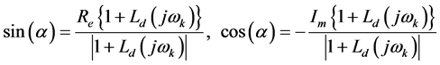
As it is well known,  is the critical point on the Nyquist plot for analyzing the stability of the closed-loop system. The distance between the critical point and the open-loop transfer function is
 . In Figure 1 the robust performance condition in (6) is met if and only if the Nyquist plot of a circle with radius
  centered at
  does not intersect with a circle (uncertainty circle) centered at
  with radius
  for all
  [9] . The line d as shown in Figure 1 is tangent to the circle cen-

Figure 1. Linear constraints on Nyquist plot.
tered at the critical point and orthogonal to the line that connects the center of the critical point to the desired open-loop transfer function . A sufficient condition for (6) is that the uncertainty circle lies at the side of d that excludes the critical point for all frequencies. The line d has infinite number of points and each point can be represented as a point in the complex plane, has real part x and imaginary part y. At each frequency
  (each point) the equation of the line d can be written as:
 (7)
(7)
where  and
and  are functions of
 , x and y are the real and imaginary parts on a point complex plane.
So the equation of the line d in (7) can be rewritten as:
 (8)
(8)
The side of the line d that excludes the critical point can be given by the following linear constraints:
 (9)
(9)
The linear constraints in (9) can be simplified by using the following facts:
 and
and 
The new linear constraints in (9) will be
 (10)
(10)
where  stands for the complex conjugate of
 .
.
In order for this condition to be satisfied for a set of uncertainty models, the uncertainty circle centered at  should be approximated by a polygon of
  vertices. Then, to satisfy the robust condition in (5) all the vertices of the polygon have to be located on the right side of the line d. This condition can be represented by the linear constraints on (11):
 (11)
(11)
where , and
, and
 (12)
(12)
Using all the above analysis, the quadratic optimization problem can be formulated as given in (13).
 (13)
(13)
Subject to:

for  (No. of frequencies),
where 
2.2. Choice of the Desired Open-Loop Transfer Function (Ld)
Selecting the desired open-loop transfer function should be based on considering plant, desired specifications and the structure of the designed controller. The desired open-loop transfer function  typically has a large amplitude in low frequencies (for good performance in tracking and disturbance rejection) and small amplitude in high frequencies for robustness with respect to unmodeled dynamics. A very typical choice for
  is
is  where
where  the desired closed-loop bandwidth. It is clear that
  is large in low frequencies and small in high frequencies and crosses the 0 dB axis at the crossover frequency
 , which ensures a closed loop bandwidth equal to
  [7] [9] .
2.3. The Controller Design Procedure
The steps of designing the proposed controller are:
1) Selecting different operating points. For case study, three operating points are given in Table 2.
2) Selecting a desired open-loop transfer function , typically equal to
 .
.
3) Solving the convex optimization problem in (13) to find an initial controller .
.
4) The results may be improved if different desired open-loop transfer function is used for each model. In this case  can be chosen.
5) The new desired open-loop transfer function  is used to design a new controller K for all the operating points.
3. Test System
3.1. Tow Area Four Machines Test System
The two-area four-machine test system is considered as one of the standard models that have been used to study the inter-area oscillations phenomenon. The test power system consists of two areas connected through two parallel tie lines and each area consists of two synchronous generators as shown in Figure 2. The generators of Area 1 (G1 and G2) are rated at 700 MW, and the generators of Area 2 (G3 and G4) are rated at 719 MW, and 700 MW, respectively. The four generators are equipped with automatic voltage regulators power system stabilizers, and turbine governors. The tie line power flow from Area 1 to Area 2 at the steady state is 400 MW. The SVC is installed at bus 8. The complete system data can be found in [10] .
3.2. Static VAR Compensator
SVC has been integrated in the test system. SVC is a shunt FACTS device that has been used to inject reactive current into the system at the point of connection. It is mainly used to improve voltage stability of the power system. SVCs can also be used for damping inter-area oscillations which can be achieved by adding a supplementary control signal to the voltage reference point of a SVC [5] . The location of SVCs in an interconnected power system might be at the sending end or receiving end of long tie-lines. The block diagram of the SVC that used in this paper is shown in Figure 3(a). The aim is to damp tie line oscillations using the SVC supplementary signal.
Table 1 shows the eigenvalue pair, the frequency and the damping ratio which represent the inter-area mode at the normal operating point . The measured signal y is the tie-line power through the line 7 - 8 which is used as an input to the controller K(s) as shown in Figure 2. The output signal of the supplementary controller u is used to provide supplementary signal to the reference of the SVC. Therefore, the control system can be represented as shown in Figure 3(b). The parameters for the SVC are given in the Appendix.
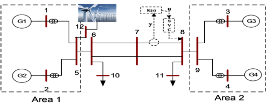
Figure 2. Single line diagram of two-area four-machines test system.

 (a) (b)
Figure 3. (a) The block diagram of an SVC; (b) The control representation of the system.

Table 1. Eigenvalue, damping ratio and the frequency of the test system.
3.3. DFIG Model
In this work, the third order model of a doubly fed induction generator is used. The dynamic modeling of the DFIG involves a set of differential algebraic equations [11] which has been built in PST [12] [13] . The model has been verified under large and small disturbances by comparing the time domain result with PSAT software. The wind turbine is installed in area 1 at bus 12 as shown in Figure 2.
4. Simulation Results for the Case Study
4.1. Control Design
Three operating points (2, 4 and 5) as shown in Table 2 are selected to design the initial controller  and the rest of the operating points are selected to test the robustness of the system. Both
  and
and  are used to calculate the new open-loop transfer function
  for all the models which is needed to design
 . The parameter of Laguerre basis is chosen as
  and the order of the controller is considered to be 3. The desired closed-loop bandwidth is
 , so the desired open loop transfer function is chosen (based on [9] ) as
 . This choice is suitable for damping the desired inter-area modes. Tuned weighting filters
  as a low pass filter and
  as high pass filter are shown in (14). The transfer function of the designed third order controller is shown in (15).
 (14)
(14)
 (15)
(15)
4.2. Two-Area Test System under Different Load Conditions
The two-area system is studied under different operating points (load conditions shown in Table 2) and fault conditions with and without the SVC supplementary controller . All the values in Table 2 are in per unit system based on 100 MVA. In this section the output power of the wind is kept constant at 300 MW.
4.2.1. The Controller Response to Different Load Conditions and Uncertainty in the System
To test the robustness of the test system, a three-phase to ground fault is applied at different locations (bus 6 and bus 8) and it is cleared (self-cleared) after 50 ms at different load conditions (points No. 1*, 4, and 6*) as shown in Table 2. As it has been mentioned the operating pint 4 is selected as one of the three operating points that the controller has been designed based on. On the other hand, the points 1* and 6* are selected as new load condition scenarios to see if the controller can maintain the robustness under these unconsidered points in the controller design. Figures 4(a)-(d) show the time domain results of the tie-line power in line 7 - 8 of the three operating
Table 2. Different operating points for two-area test system.
*It is not used in the control design, it is used to validate the controller.
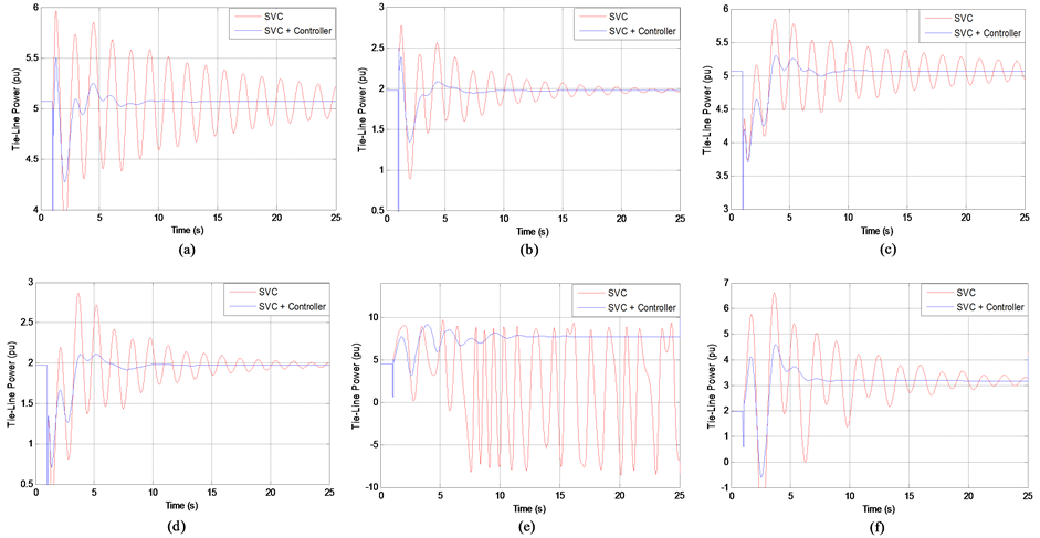
Figure 4. Tie-line power at different, load conditions, fault locations and change in system topology. (a) 480 MW tie-line, fault at bus 6; (b) 200 MW tie-line, fault at bus 6; (c) 480 MW tie line, fault at bus 8; (d) 200 MW tie line, fault at bus 8; (e) 480 MW tie-line, trip the line 6 - 7; (f) 200 MW tie-line, trip the line 6 - 7.
points under three phase fault applied at bus 6 and bus 8. It can be seen that, the controller can maintain the robustness under different load conditions. Also, without the supplementary controller the oscillations need more time to be damped compared to the system with the controller.
4.2.2. The Controller Response to Changes in System Topology
The change in system topology has been achieved by applying three phase fault at bus 7 and clearing the fault by tripping the line 6 - 7. Figure 4(e) and Figure 4(f) show the tie-line power in line 7 - 8 at different load conditions under tripping the above line. The system cannot maintain the stability without the supplementary controller when the tie-line power between the two areas increased to be almost 500 MW as show in Figure 4(e); however, the stability can be maintained by adding the supplementary controller and that makes the system more robust. Adding the supplementary controller not only helps to damp the inter-area oscillations, it gives more flexibility to exchange the power between the two areas.
4.3. Two-Area Test System under Different Wind Penetrations
4.3.1. The Controller Response to Different Wind Penetrations and Uncertainty
The wind penetrations are changed according to the weather conditions and that affects the robustness of the system. The designed controller is tested under different levels of wind penetrations. Three different levels of wind penetrations (300, 200 and 100 MW) are selected to show the impact of wind power penetration on the robustness of the test system. Figures 5(a)-(c) show the tie-line power under different operating points when the level of the wind penetration is equal to 200 MW and 100 MW. The simulation results illustrate that, the supplementary controller is able to damp the oscillations within 5 sec under different load conditions.
4.3.2. The Controller Response to Changes in System Topology
The performance of the designed controller has been examined under tripping the line 7 - 8 at different level of wind penetrations. Figures 5(d)-(f) show the tie-line power in line with 200 MW and 100 MW wind under different load conditions. The controller can maintain the stability under this outage which makes the system more robust.
4.4. Eigenvalue Analysis
Eigenvalue study has been done to examine the performance of the supplementary controller in terms of improving the damping ratio ξ of the inter-area modes. The results are concluded in Table 3. It can be seen that the damping ratios of different load conditions are improved.
Table 4 summarized the damping ratios of the inter-area modes under different level of wind penetrations

Figure 5. Tie-line power at different wind penetrations and change in system topology. (a) 400 MW, 200 MW wind, fault at bus 6; (b) 300 MW, 200 MW wind, fault at bus 6; (c) 300 MW, 100 MW wind, fault at bus 6; (d) 300 MW, 200 MW wind, trip the line 6 - 7; (e) 300 MW, 100 MW wind, trip the line 6 - 7; (f) 100 MW, 100 MW wind, trip the line 6 - 7.
Table 3. Damping and frequencies of the inter-area modes under different load conditions.
Table 4. Damping and frequencies under different wind penetrations.
( ). The results show that the action of the supplementary controller is robust against varying the level of the wind penetrations. It can be seen that when the penetration level is decreased to 50 MW the system becomes unstable (negative damping ratio) without the controller.
5. Conclusion
A new method was introduced and implemented in this paper to design a robust fixed-order  controller. The basic concept of the
  design has been detailed. Basically this approach is based on shaping the open- loop transfer function in the Nyquist diagram. The performance of the designed controller has been evaluated under different load conditions as well as different levels of wind penetrations. One of the advantages of the proposed approach is that it does not need the system to be reduced. For example, the two-area test system with wind has 75 states and only 3-order controller is required. The main advantage of the proposed method is considering the multi-model uncertainty. The results show that the designed controller is robust and helps the system to maintain the stability under small and large disturbances. In some cases, the system loses the stability without the supplementary controller. It can be concluded that the controller is robust respect to changes in the load conditions as well as different levels of wind penetrations.
Cite this paper
Abdlmnam Abdlrahem,Parimal Saraf,Karthikeyan Balasubramaniam,Ramtain Hadidi,Alireza Karimi,Elham Makram, (2016) Design of a Fixed-Order Robust Controller to Damp Inter-Area Oscillations in Power Systems. Journal of Power and Energy Engineering,04,61-70. doi: 10.4236/jpee.2016.43006
References
- 1. Chaudhuri, B. and Pal, B. (2004) Robust Damping of Multiple Swing Modes Employing Global Stabilizing Signals with a TCSC. IEEE Transactions on Power Systems, 19, 499-506.
http://dx.doi.org/10.1109/TPWRS.2003.821463 - 2. Chaudhuri, B., Pal, B., Zolotas, A.C., Jaimoukha, I.M. and Green, T.C. (2003) Mixed-Sensitivity Approach to H Control of Power System Oscillations Employing Multiple Facts Devices. IEEE Transactions on Power Systems, 18, 1149- 1156.
http://dx.doi.org/10.1109/TPWRS.2003.811311 - 3. Klein, M., Le, L., Rogers, G., Farrokpay, S. and Balu, N. (1995) H Damping Controller Design in Large Power System. IEEE Transactions on Power Systems, 10, 158-166.
http://dx.doi.org/10.1109/59.373938 - 4. Majumder, R., Pal, B.C., Dufour, C. and Korba, P. (2006) Design and Real-Time Implementation of Robust FACTS Controller for Damping Inter-Area Oscillation. IEEE Transactions on Power Systems, 21, 809-816.
http://dx.doi.org/10.1109/TPWRS.2006.873020 - 5. Zhao, Q. and Jiang, J. (1995) Robust SVC Controller Design for Improving Power System Damping. IEEE Transactions on Power Systems, 10, 1927-1932.
http://dx.doi.org/10.1109/59.476059 - 6. Chen, S. and Malik, O. (1995) Power System Stabilizer Design Using Synthesis. IEEE Transactions on Energy Conversions, 10, 175-181.
http://dx.doi.org/10.1109/60.372584 - 7. Karimi, A. (2013) Frequency-Domain Robust Control Toolbox. 52nd Conference in Decision and Control, Florence, Italy, 10-13 December 2013, 3744-3749.
http://dx.doi.org/10.1109/CDC.2013.6760460 - 8. Galdos, G. (2010) Fixed-Order Robust Controller Design by Convex Optimization Using Spectral Models. Thèse EPFL, No. 4785.
- 9. Karimi, A. and Galdos, G. (2010) Fixed-Order H∞ Controller Design for Nonparametric Models by Convex Optimization. Automatica, 46, 1388-1394.
http://dx.doi.org/10.1016/j.automatica.2010.05.019 - 10. Kundur, P. (1994) Power System Stability and Control. McGraw-Hill, New York.
- 11. Milano, F. (2005) Power System Analysis Toolbox.
- 12. MathWorks Inc. (2014) MATLAB Version 8.3.0.532.
- 13. Cherry Tree Scientific Software (1991-2008) Power System Toobox ver. 3.0.
Appendix
SVC Parameters:
 ,
,
 ,
,
 ,
,
 ,
,
 ,
,
 ,
,
 .
.