Received 24 August 2015; accepted 25 October 2015; published 28 October 2015

ABSTRACT

This study is concerned with the numerical approximation of the extended Fisher-Kolmogorov equation with a modified boundary integral method. A key aspect of this formulation is that it relaxes the domain-driven approach of a typical boundary element (BEM) technique. While its discretization keeps faith with the second order accurate BEM formulation, its implementation is element-based. This leads to a local solution of all integral equation and their final assembly into a slender and banded coefficient matrix which is far easier to manipulate numerically. This outcome is much better than working with BEM’s fully populated coefficient matrices resulting from a numerical encounter with the problem domain especially for nonlinear, transient, and heterogeneous problems. Faithful results of high accuracy are achieved when the results obtained herein are compared with those available in literature.

Keywords:

Boundary Element Method, Extended Fisher-Kolmogorov Equation Boundary Integral Formulation, Slender Coefficient Matrix, Hybridization, Domain-Driven

1. Introduction

The major thrust of the paper is a numerical study of a nonlinear fourth order partial differential equation in a hybrid boundary integral setting.

Many problems in engineering and applied sciences can be represented by fourth order differential equations. A good understanding of the processes that lead to their derivation can only be obtained via numerical solutions. Several examples of these can be found in scientific literature for example, the Euler-Bernoulli beam theory equation [1] which gives the transverse deflection of a cantilever beam under a uniform transverse load or the EFK equation, a fourth order partial differential equation used for the study of several physical phenomena for example travelling waves in reaction-diffusion systems [2] , physical systems that are bi-stable, pattern formation, as well as instability in nematic fluid crystals. The one-dimensional version of this equation has been studied extensively by Danumjaya [3] where he showed the existence and uniqueness results for weak solutions by using Lyapunov function.

Earlier work by Danumjaya and Pani [4] involved the splitting of EFK equation into two second order equations and subsequent application of the orthogonal cubic spline collocation (OSC) method. This was followed by the study of travelling waves in reaction diffusion systems (Zimmerman [5] and Aronson and Weinberger [6] ). Peletier and Troy [7] studied the steady state version of EFK equation using the shooting method. Periodic solutions were discussed by Peletier et al. [8] and Stepan and Julia [9] , while qualitative work was carried out by Hung Luo [10] who looked at the global attractors of the EFK equation in H^k spaces. Extensive analysis in this field has been recorded (Kalies et al. [11] , Noomen and Omrani [12] as well as Kadri and Omrani [13] ).

However a review of current literature clearly demonstrates paucity of information on the application of the boundary integral method to the numerical solution of the EFK equation. The reason is not far-fetched and primarily arises from several factors among which are its transient nature, its fourth order, its dimensionality and nonlinearity. These are factors which pose serious numerical challenge to a typical BEM formulation. The hybrid boundary integral technique applied herein is able to deal satisfactorily with these problems [14] [15] by splitting the differential equation into a two coupled system and applying a hybrid procedure based on a boundary integral formulation.

This approach is initiated by transforming the governing differential equation into its integral analog via the Green’s second identity followed by a FEM-like element-by-element implementation of the resulting equations throughout the problem domain. Unlike other BEM techniques, no extraneous mathematical techniques are applied to do all integration on the boundary of the problem domain. The whole process is amply simplified by the presence of a source point inside a generic element which facilitates a “local support” based numerical integration akin to the FEM implementation. The gain resulting from this approach is immense because the resulting integral equations appear in the form of local element equations whose contributions add up to produce slender and banded coefficient matrices [16] [17] .

A lot of effort has been expended in dealing with domain integrals arising from BEM implementation (Portapila and Power [18] , Hibersek and Skerget [19] ). These have been principally directed towards dealing with this undesirable feature of BEM formulation. BEM literature is replete with several surrogate varieties of BEM with numerous mathematical artifacts aimed at facilitating a boundary-only version of BEM implementation. Sladeck et al. [20] applied temporal free space Green functions in two spatial dimensions to model transport equations for low values of Peclet number. The development of accurate BEM numerical procedures for effectively handling both the problem domain as well as its boundary is a task that is just beginning (Archer et al. [21] , Grogoriev [22] , Perrata and Popov [23] ).

2. Numerical Formulation

The EFK equation is given by

(1)

where, subject to initial condition

(2)

and boundary conditions

(3)

(4)

We apply a splitting technique by converting Equation (1) into a two coupled system of differential equations.

(5)

and Equation (1) becomes

(6)

with the following change in one of the boundary conditions

(7)

Numerical approximation of Equations (5) and (6) in line with a hybrid boundary integral implementation involves the following steps:

1) We seek the solution of a prescribed auxiliary differential equation of a governing differential equation. This solution (fundamental solution or the free space Green function) constitutes a key element for obtaining the integral analog of the governing differential equation via the Green’s second identity.

2) Classical BEM approach requires that any part of the governing differential equation that does not contribute to the auxiliary differential equation is treated as a boundary integral in the “integralization” procedure. This is the origin of most of the numerical difficulties encountered in BEM numerical implementation. The implication here is that various components of a differential equation whose physics dictates direct interaction with the problem domain are forced to the boundary. We refer to body force terms, heterogeneity, nonlinearity, temporal terms etc. The hybrid method employed herein does not consider domain integration as a disadvantage because it is domain-element-driven. As a result the ensuing computations are relatively straightforward.

3) The finite element component of the hybrid formulation demands that dicretization be carried out throughout the problem domain, with initial and boundary conditions satisfied as well as the enforcement of inter element continuity. Finally all element equations are assembled to form a global coefficient matrix. These are slender and banded because the procedure takes advantage of the “local support” inherent in the finite element formulation.

4) The resulting coefficient matrix together with the right hand side vector of known values (boundary and initial conditions and specified problem parameters) is solved to yield the problem dependent variables. We hasten to comment that boundary element formulation of the hybrid algorithm guarantees a second order accuracy in the computed results.

Numerical discretization of the coupled system is sought by specifying a suitable complementary differential equation whose solution straightforward to obtain. A good example of this follows from previous work [24] [25] and is given by

(8)

where G is the Green’s function and the Dirac delta forcing function. A well known fundamental solution of (8) is given by where is an arbitrary function and usually taken as the longest element used for discretizing the problem domain. The derivative of the fundamental solution is represented as: where is the Heaviside function with the property

(9)

Substitution of the complementary equation, its fundamental solution, and its derivative into the Green’s second identity provides a platform for transforming the governing differential equation into its integro-differ- rential analogs. Without any loss of generality these can be represented by:

(10a)

(10b)

(10c)

where is the primary variable and is its spatial derivative, is a constant that takes a value of 0.5 or unity depending on whether the source point is located within or at the boundaries of the problem domain. Interpolation for all the terms within the integrals yields:

(11a)

(11b)

where is a linear interpolation function with respect to an element node j. When appropriate substitutions are made, and a finite difference temporal discretization implemented, we obtain a general system of transient, discrete equations including reaction, nonlinear source terms of the type shown below.

(12)

The nonlinearity in Equation (12) can be resolved by the Newton-Raphson or Picard schemes [15] [16] .

2.1. Numerical Experiments

In this section we apply the method developed herein to numerically solve the extended Fisher-Kolmogorov equation and compare the displayed results with those available in literature.

2.1.1. Example 1

We consider the EFK Equation (1) with the following boundary and initial conditions:

(13)

and initial condition

(14)

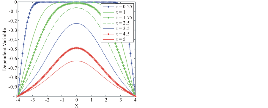
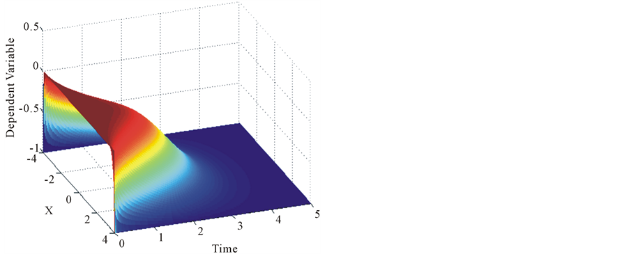
The numerical solution of the governing differential equation has been found for at different times with. Figure 1(a) displays the numerical solutions at different times and all are found to be in excellent agreement with those of Mittal and Arora [26] and in addition confirms that for a small initial data, the solution decays nonlinearly as time increases and finally approaches a value of unity at both boundaries. Figure 1(b) shows a 3-D graph of the solution profile and confirms that the longer the numerical solution the less steep the solution profile and the more the decay of the dependent variable as they all approach a value of unity.

2.1.2. Example 2

The problem is specified to read:

(15)

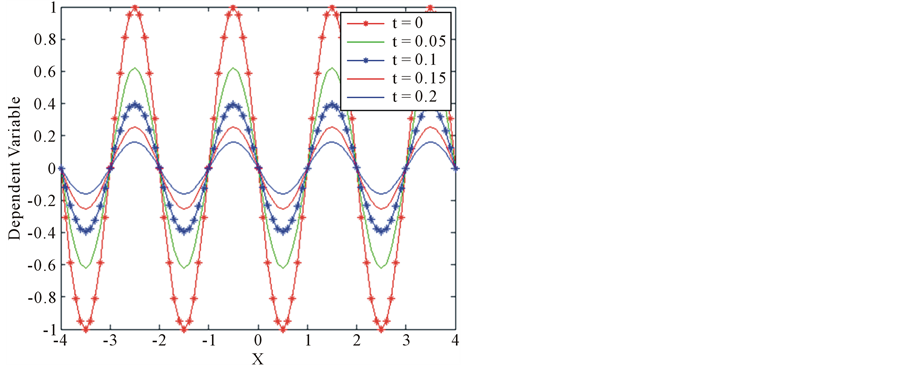
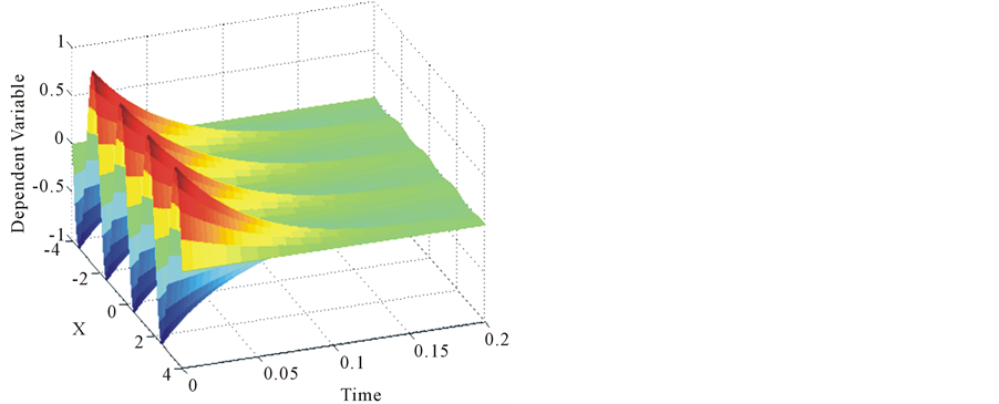
The initial condition as well as the problem parameters is left the same. Figure 2(a) shows results that are consistent with those of Mittal and Arora [26] . Figure 2(b) also confirms that as time increases, the scalar profiles approach −1.

2.1.3. Example 3

This problem is taken from Danumjaya and Pani [4] . The boundary and initial conditions are given as:

(16)

and an initial condition given by

(17)

Changing the value of gamma from to makes the solution profile to decay relatively very fast. This illustrates the stabilizing influence of the parameter in the EFK equation and shows agreement between Figure 3(a) and Figure 3(b) with those of Figure 1 and Figure 2 of [4] . A display of the flatter slopes in Figure 3(d) when compared with those of Figure 3(c) help to confirm this observation.

2.2. Convergence Test (in Table 1)

The exact solutions of the EFK equation for the given initial and boundary conditions are not known. In order for us to have meaningful tests, the exact solution is replaced with the EFK numerical solution for 160 partitions and the numerical solutions at different intervals are compared with these. To this end, the following parameters are applied.

where is the error with number of segments and the error in this sense can be interpreted as as defined above.

3. Conclusion

We have demonstrated a straightforward hybrid BEM approach for solving a fourth order nonlinear equation of considerable significance in mathematical physics. The approach demonstrated here is simple and straightforward and involves the splitting of the governing differential equations into two second order components followed by an application of BEM-FEM numerical procedure. The utility of the present formulation rests on the fact that all integrations are performed locally and a slender coefficient matrix is created by assembling all local solutions. This approach facilitates the handling of some of the notorious disadvantages that plague the direct BEM formulation and pave the way for more challenging computations.

Cite this paper

Okey OselokaOnyejekwe, (2015) A Direct Implementation of a Modified Boundary Integral Formulation for the Extended Fisher-Kolmogorov Equation. Journal of Applied Mathematics and Physics,03,1262-1269. doi: 10.4236/jamp.2015.310155

References

- 1. Onyejekwe, O.O. (2004) A Green Element Method for Fourth Order Differential Equations. Advances in Engineering Software, 35, 517-525.
http://dx.doi.org/10.1016/j.advengsoft.2004.05.005 - 2. Dee, G.T. and Van Sarloos, W. (1988) Bistable Systems with Propagating Fronts Leading to Pattern Formation. Physical Review Letters, 60, 2641-2644.
http://dx.doi.org/10.1103/PhysRevLett.60.2641 - 3. Danumjaya, P. and Pani, A.K. (2006) Numerical Methods for Extended Fisher-Kolmogorov (EFK) Equation. International Journal of Numerical Analysis and Modeling, 3, 186-210.
- 4. Danumjaya, P. and Pani, A.K. (2005) Orthogonal Cubic Spline Collocation Method for the Extended Fisher Kolmogorov (EFK) Equation. Journal of Computational and Applied Mathematics, 174, 101-117.
http://dx.doi.org/10.1016/j.cam.2004.04.002 - 5. Zimmerman, W. (1991) Propagating Fronts near a Lifshitz Point. Physical Review Letters, 66, 1546.
http://dx.doi.org/10.1103/PhysRevLett.66.1546 - 6. Aronson, D.G. and Weinberger, H.F. (1978) Multidimensional Nonlinear Diffusion Arising in Population Genetics. Advances in Mathematics, 30, 33-67.
http://dx.doi.org/10.1016/0001-8708(78)90130-5 - 7. Peletier, L.A. and Troy, W.C. (1995) A Topological Shooting Method and Existence of Kinks of the Extended Fisher-Kolmogorov Equation. Topological Methods in Nonlinear Analysis, 6, 331-355.
- 8. Peletier, L.A., Troy, W.C. and Vander Vorst, R.C.A.M. (1995) Stationary Solutions of a Nonlinear Fourth Order Equation. Differential Equations, 31, 327-337.
- 9. Tersian, S. and Chaparova, J. (2001) Periodic and Homoclinic Solutions of Ex-tended Fisher Kolmogorov Equations. Journal of Mathematical Analysis and Applications, 260, 490-506.
http://dx.doi.org/10.1006/jmaa.2001.7470 - 10. Hong, L. (2011) Global Attractor of the Extended Fisher-Kolmogorov Equation in Hk Spaces. Boundary Value Problems, 2011, 39.
http://dx.doi.org/10.1186/1687-2770-2011-39 - 11. Kalies, W.D., Kwapisz, J. and VanderVorst, R.C.A.M. (1996) Homotopy Classes for Stable Connections between Hamiltonian Saddle-Focus Equilibria. Preprint of Georgia Tech.
- 12. Noomen, K. and Omrani, K. (2011) Finite Difference Discretization of the Extended Fisher-Kolmogorov Equation in Two Dimensions. Computers & Mathematics with Applications, 62, 4151-4160.
http://dx.doi.org/10.1016/j.camwa.2011.09.065 - 13. Kadri, T. and Omrani, K. (2011) A Second Order Accurate Difference Scheme for an Extended Fisher-Kolmogorov Equation. Computers & Mathematics with Applications, 61, 451-459.
http://dx.doi.org/10.1016/j.camwa.2010.11.022 - 14. Taigbenu, A.E. and Onyejekwe, O.O. (1997) A Mixed Green Element Formulation for Transient Burgers’ Equation. International Journal for Numerical Methods in Fluids, 24, 563-578.
- 15. Onyejekwe, O.O. (2015) An Hermitian Boundary Integral Hybrid Formulation for Nonlinear Fisher-Type Equations. Applied and Computational Mathematics, 4, 83-99.
http://dx.doi.org/10.11648/j.acm.20150403.11 - 16. Onyejekwe, O.O. and Onyejekwe, O.N. (2013) A Nonlinear Integral Formulation for a Stream Aquifer Interaction Flow Problem. International Journal of Nonlinear Science, 15, 15-26.
- 17. Bagherinezhad, A. and Pishvaie, M.R. (2014) A New Approach to Counter-Current Spontaneous Imbibition Simulation Using Green Element Method. Journal of Petroleum Science and Engineering, 119, 163-168.
http://dx.doi.org/10.1016/j.petrol.2014.05.004 - 18. Portapila, M. and Power, H. (2008) Iterative Solution Schemes for Quadratic DRM-MD. Numerical Methods for Partial Differential Equations, 24, 1430-1459.
- 19. Hibersek, M. and Skerget, L. (1996) Domain Decomposition Methods for Fluid Flow Problems by Boundary Integral Method. Zeitschrift fur Angewandle Mathematik und Mechanik, 76, 115-139.
- 20. Sladeck, J., Sladeck, V. and Zhang, C. (2004) A Local BIEM for Analysis of Transient Heat Conduction with Nonlinear Source Terms in FMG’s. Engineering Analysis with Boundary Elements, 28, 1-11.
- 21. Archer, R., Horne, R.N. and Onyejekwe, O.O. (1999) Petroleum Reservoir Engineering Applications of the Dual Reciprocity Boundary Element Method and the Green Element Method. 21st World Conference on Boundary Element Method, 25-27 August 1999, Oxford University, Eng-land.
- 22. Grigoriev, M.M. and Dargush, G.F. (2003) Boundary Element Methods for Transient Convective Diffusion Part 1: General Formulation and 1D Implementation. Computer Methods in Applied Mechanics and Engineering, 192, 4281-4298.
- 23. Peratta, A. and Popov, V. (2004) Numerical Stability of the BEM for Advection-Diffusion Problems. Numerical Methods for Partial Differential Equations, 20, 675-702.
http://dx.doi.org/10.1002/num.20009 - 24. Onyejekwe, O.O. (2000) Experiences in Solutions of Nonlinear Transport Equations with Green Element Method. International Journal of Numerical Methods for Heat & Fluid Flow, 10, 675-686.
http://dx.doi.org/10.1108/09615530010350372 - 25. Onyejekwe, O.O. (1999) Numerical Properties of Green Element Unsteady Transport. Transactions on Modelling and Simulation, 24, 749-758.
- 26. Mittal, R.C. and Arora, G. (2009) Quintic B-Spline Collocation Method for Numerical Solution of the Extended Fisher-Kolmogorov Equation. International Journal of Applied Mathematics and Mechanics, 6, 74-85.