Open Journal of Modern Hydrology
Vol.3 No.1(2013), Article ID:27244,12 pages DOI:10.4236/ojmh.2013.31006
Effect of Terrestrial LiDAR Point Sampling Density in Ephemeral Gully Characterization
![]()
1Department of Geosciences, Middle Tennessee State University, Murfreesboro, USA; 2National Sedimentation Laboratory, United States Department of Agriculture—Agricultural Research Service, Oxford, USA; 3United States Department of Agriculture—Natural Resources Conservation Service, Salina, USA.
Email: *henrique.momm@mtsu.edu
Received November 27th, 2012; revised December 30th, 2012; accepted January 9th, 2013
Keywords: Ephemeral Gully; Ground-Based LiDAR; Soil Erosion; Point Sampling Density; Remote Sensing
ABSTRACT
Gully erosion can account for significant volumes of sediment exiting agricultural landscapes, but is difficult to monitor and quantify its evolution with traditional surveying technology. Scientific investigations of gullies depend on accurate and detailed topographic information to understand and evaluate the complex interactions between field topography and gully evolution. Detailed terrain representations can be produced by new technologies such as terrestrial LiDAR systems. These systems are capable of collecting information with a wide range of ground point sampling densities as a result of operator controlled factors. Increasing point density results in richer datasets at a cost of increased time needed to complete field surveys. In large research watersheds, with hundreds of sites being monitored, data collection can become costly and time consuming. In this study, the effect of point sampling density on the capability to collect topographic information was investigated at individual gully scale. This was performed through the utilization of semivariograms to produce overall guiding principles for multi-temporal gully surveys based on various levels of laser sampling points and relief variation (low, moderate, and high). Results indicated the existence of a point sampling density threshold that produces little or no additional topographic information when exceeded. A reduced dataset was created using the density thresholds and compared to the original dataset with no major discrepancy. Although variations in relief and soil roughness can lead to different point sampling density requirements, the outcome of this study serves as practical guidance for future field surveys of gully evolution and erosion.
1. Introduction
In agricultural fields, gully erosion is significant and often similar to or exceeding sheet and rill erosion volume. A large number of modeling tools have been developed over the years to estimate sediment transport from agricultural fields to streams and lakes [1-3]. These tools play an important role in assessing existing and planned conservation practices and are accepted by various regulatory and management agencies such as the United States Environmental Protection Agency (EPA) and the United States Natural Resource Conservation Service (NRCS). However, at the current stage of development, sediment loss estimation from gullies is either limited or neglected. Unlike sheet and rill erosion, which occurs as a result of the impact of raindrops and water flowing on the soil surface, gully erosion in agricultural fields occurs as a result of concentrated flow of surface runoff along a defined channel, and also by subsurface flow by seepage and flow through preferential pathways [4]. Gullies in agriculture fields are often classified into either ephemeral or classical gullies.
Ephemeral gullies are defined as small channels located in agricultural fields eroded primarily from concentrated overland flow that can be easily filled by normal tillage, only to reform again in the same location by additional runoff events [5]. Due to their small dimensions, producers often reshape the channel’s topography, by refilling the channel through tillage, to maintain regular farming operations [6]. Because the field topography is often unchanged between seasons, ephemeral gullies have a tendency to re-form at the same or nearby location [7]. An ephemeral gully becomes permanent, referred to as classic gully, in situations where a headcut migrates upstream faster than the time interval between farmers tilling operations, followed by widening of the channel and which forces producers to operate around the gully channel.
This dynamic behavior poses a challenge in the understanding and estimation of the soil erosion of ephemeral gullies in agricultural watersheds [7]. Studies designed to understand ephemeral gully formation and development typically use Digital Elevation Models (DEM) as the basis of formulations explaining the relationship between field topography and ephemeral gully occurrence [8-10]. Despite the availability of DEMs at regional and local scales (spatial resolution ranging from 1 to 30 meters), these datasets often do not offer the necessary spatial resolution to quantify gullies at field scales. In order to capture the micro-topography impacting ephemeral gully formation, DEMs with spatial resolution ranging between 5 mm to 5 cm have found to be necessary [11]. Digital representations at such a detailed scale provide the necessary information to accurately quantify ephemeral gully soil loss and channel morphology.
Recent developments in laser scanner technology, provides new opportunities for scientific investigation of ephemeral and classical gullies. Although, laser scanners have been previously used in similar investigations such as large-scale classical gullies in different locations such as mountain-side sites [12], forest sites [13], desert sites [14], and landslides [15,16], its application to ephemeral gully investigations is in the early stages of development. This can be partially attributed to the dynamic nature and small scale of ephemeral gullies that limit the identification and description of such features using airbornebased Light Detection And Ranging (LiDAR) systems. Due to reduced cost and increased portability of laser scanner technology, terrestrial LiDAR surveys are now practical.
Ground-based LiDAR systems provide the tools for detailed multi-temporal analysis of micro-topography of ephemeral gullies. These systems are capable of generating terrain representations with sub-centimeter vertical accuracy (Table 1). This is especially important in research sites where the same location needs to be surveyed multiple times over lengthy intervals as conditions change due to precipitation, runoff events, field management changes, and/or implementation of conservation practices. However, as the number of data points increase (point sampling density) with increased resolution-rich surveys, so does the time required for field data collection, post processing, and the size of datasets. This problem is compounded when monitoring multiple sites with different topographic and farming practices. The objecttive of this study is to identify the minimum point sampling density that provides the necessary topographic information to efficiently produce reproducible field surveys. The results of this study may be used as a guideline in using laser scanner technology to characterize topographic conditions associated with the evolution of ephemeral and classical gullies and, more importantly, accurate estimates of quantities of sediment eroded or conserved by erosion control practices.
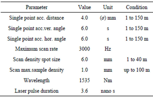
Table 1. General specifications of the TOPOCON GLS-1000 laser scanner.
2. Background
2.1. Point Sample Density
LiDAR technology measures the laser pulse travel time from the transmitter to the target and back to the receiver [17]. Because the speed of light is a known constant, the distance can then be calculated. In this process, a very accurate timing system is needed to guarantee precise estimates since the laser pulses are generally sent at the rate of thousands of times per second. Additionally, the transmitter and the receiver must be located at the same physical location, so in effect containing a single-ended system [18]. During the field data collection process, ground-based laser scanners record vertical and horizontal angles, intensity of the returned signal, and the traveled distance for each laser pulse.
These systems are capable of collecting information with a wide range of ground point sampling densities as a result of operator controlled factors such as the scan angles (area covered by individual scans), average point density of individual scans, and degree of overlap between scans (Figure 1). Higher point density can be achieved by higher sensor resolution, smaller vertical field of view angles, and multiple scans of the same ground location. The instrument resolution is often controlled by an imaginary plane located at the middle range of the vertical field of view and is orthogonal to the sensor’s normal sight. The vertical scan angle also influences sampling density. Surveying with large vertical angles covers more area and often yields shorter survey times, but at the expense of point sampling density (see Figure 1). Multiple scans can be used to collect data over the same geographical location resulting in increased sampling density and often overcomes problems such as shadowing and limited coverage due to vegetation.
2.2. Spatial Variability
Modeling tools designed to define and to understand the pathways of surface water movement across fields and even across watersheds rely on raster-based digital elevation models to derive the required topographic attributes [19]. The conversion of irregularly spaced and uneven distributed laser points into a regularly spaced grid requires the use of interpolation and re-sampling techniques. The choice of a specific interpolation method and its corresponding parameters introduce uncertainties that are propagated to the hydrologic model [19] and studies have been conducted to study such phenomena [20].
Among all the available interpolation techniques, kriging is often used because of the ability to provide unbiased estimates with minimum and known variance [21]. The core element of kriging interpolation techniques is the variogram. The variogram explores spatial independence [22] and quantitatively relates variance to space separation [21]. Variogram analysis aids our understanding of the effects of scale in spatial variability on the data being interpolated.
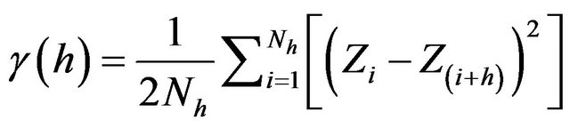
As an illustration of the variogram computation concept, consider a one-dimensional set of laser points (Figure 2). Variograms are computed using a set of pair of points, which are selected, based on a pre-defined separation distance h, referred to as lag distance. A practical equation to compute the variance of differences is the use of semivariogram equation, which is given by:
 (1)
(1)
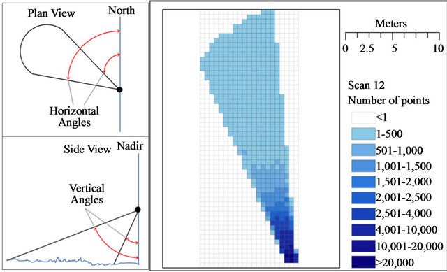
Figure 1. Illustration of spatial variation of laser point sampling density, represented as number of points per grid unit. Laser point sampling density decreases with vertical scanning angle of ground-based laser scanners.
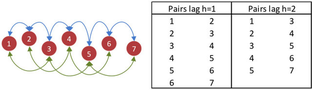
Figure 2. Conceptual illustration of the pairing of points with varying separation distance h. The list of points is used in the computation of experimental variogram.
The semivariogram equation represents the average semi-variance for a lag distance h between points and a total number of pairs Nh. In this equation Zi and Z(i + h) represent the elevation value of points at location i and i plus the separation distance h (i + h), respectively. The smaller the γ value the more related the points are. In other words, the semivariogram represents the average squared difference of any pair of points located h distance from each other [21].
Plotting semi-variance using an increasing range of lag distances generates a semivariogram graphic (Figure 3). The range of lag distances is plotted on the x-axis and the semi-variance on the y-axis. In the ideal case, points close to each other should have small difference values (small semi-variance) and as the separation distance increases the differences between points should also increase [23]. The plotted curve resulting from the semivariogram is referred to as experimental semivariogram (red points in Figure 3). When a mathematical function is used to model the experimental semivariogram it is then referred to as theoretical semivariogram. Also, in the ideal variogram two properties are regarded as the most important curve characteristics: sill and range or correlation length (Figure 3). The sill should be equal to the sample variance [24] and should match the values where the semivariogram curve “levels off”. The range, in the semivariogram plot, should correspond to the value in the x-axis matching the sill and indicates the distance where the samples become independent of each other. Experimental variograms can be considered isotropic or anisotropic, where isotropic variograms depend only on the separation distance, while anisotropic variograms depend on the separation distance and orientation. A detailed description of variograms and its role in kriging interpolations is beyond the scope of this manuscript and additional information on this topic can be found in many textbooks [23,25,26].
3. Methodology
3.1. Study Site
The study site selected for this investigation is located within the Cheney Lake Reservoir watershed near the town of Hutchinson in South Central Kansas. The predominant land use is agriculture (>73%) in the form of cropland and rangeland. The gully within the study site was 96 meters long oriented North-South, approximately 1.3 meters wide and from 10 to 50 cm deep. The channel is free of vegetation and crop residues, while the surroundings are covered by crop residues resulting from no-till management used in winter wheat followed by sorghum (milo) in the 2010 crop rotation. Historical cultivation practices indicates that initially this ephemeral gully did not disrupt farming operations; however, as no-tillage practices were adopted in 2005, the channel grew wider and deeper to the point that the farming equipment could not be used to travel across the gully and the ensuing cropping activity was performed around the main channel (Figure 4).
Two locations with known geographic coordinates within the study site were used to provide reference geographical coordinates. This is an important step to translate the equipment local coordinates into geographic coordinates, thus providing a means to compare surveys performed at different times. The equipment used was a TOPCON GSL-1000 series and its general specifications are listed on Table 1. Initially, the operator scans the pre-defined targets installed at the reference points. Based on the known geometry of the targets, the instrument is then capable of calculating its location in relation to the reference points (geographical coordinates). Four standard targets were installed in the far outmost corners of the gully being investigated. These four static targets are surveyed and their coordinates computed and recorded. Each subsequent scan starts with surveying the four targets to locate the laser scanner in the local coordinate system. A total of eleven scans in eleven set ups (one scan for each equipment set up) were used to describe the gully. In the post processing steps, each scan with local coordinates are translated into geographical coordinates using the relation between the four targets and the reference points.
3.2. Accuracy Assessment
During data collection in the field it is possible to survey the same geographical location from different scans. This practice is often used to increase sampling density and to avoid problems such as shadowing and/or limited coverage due to vegetation. The overlap in LiDAR point sampling can also be used to evaluate survey accuracy. Given that the overlapping scans were collected with enough point density, it is possible to identify neighbor ing points, collected from different scans, and compute elevation differences between these points (Figure 5). A similar approach is used to evaluate the accuracy of airborne LiDAR sensors by comparing elevation values of nearby points collected by different flight paths in overlapping areas.
Cross-validation was performed considering two distance threshold values of 1 and 5 millimeters. Histograms of the elevation difference of the selected point pairs are shown in Figure 6 and the summary statistics in Table 2. The mean difference for both cases is less than 2 cm; however, some points showed absolute differences above 5 cm. These isolated differences could be attributed to sharp elevation differences caused by features such as crop residues and standing vegetation.
3.3. Sampling Density Investigation
Studies have been performed to identify the optimum
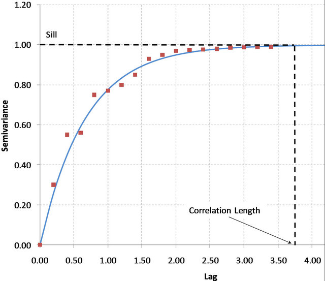
Figure 3. Ideal shape of semivariogram plot. Red squares represent the experimental semivariogram plotted from the sample data. Blue line represents the theoretical semivariogram curve obtained from fitting a mathematical model to the experimental variogram.
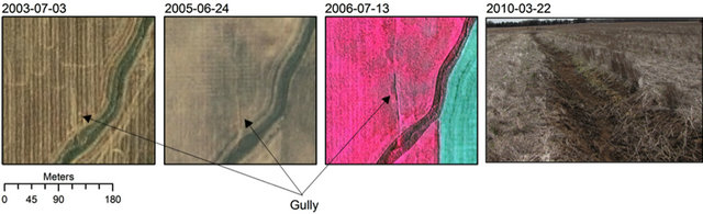
Figure 4. Ephemeral gully evolution into classical gully and its consequent disruption to producer’s operations. Imagery data for years 2003, 2005, and 2006 obtained from the National Agriculture Imagery Program (NAIP) and 2010 from field visit.
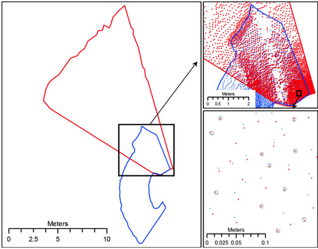
Figure 5. Overlap between different scans of ground-based LiDAR. The pair of points highlighted by a circle in the lower right map indicates the points with distances smaller or equal than 5 mm. These points were used in the survey accuracy assessment.
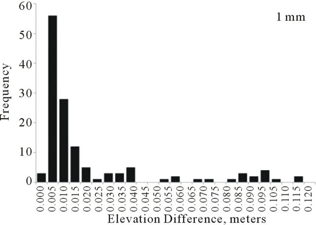
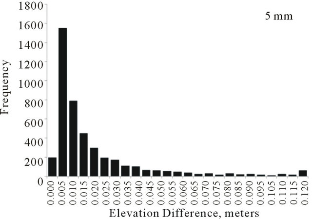
Figure 6. Histograms of elevation differences between ground-based LiDAR points collected in different scans and with distanced less 1mm (left-hand side plot) and 5 mm (right-hand side plot) apart.
balance between point density at small gully scales and volume of data with the goal of optimizing data collection and cost. Guo [20] provides a detailed investigation of the relationship associated with airborne LiDAR point density reduction, interpolation methods, and resolution of digital elevation models. There have not been studies that investigate the relationship of laser point sampling density collected using ground-based laser scanners on topographic information tailored to gully investigations in agricultural fields. Ground-based systems differ from airborne systems as a result of encountering a wider range of incidence angles [27]. Also, the finer resolution in investigations of gullies formed in agricultural fields requires the determination of micro-topography, combined with the presence of crop residues, produces various levels of terrain roughness, posing a challenge to interpolation techniques.
Point sampling density was investigated by tiling the entire LiDAR point cloud into one-meter square grids. Sampling density was computed by counting the number of points in each tile. This information can be utilized when verifying spatial coverage of sampling points to identify gaps or under-sampled regions (Figure 7). Areas with specific features, such as gully headcuts, should be scanned with higher point density, whereas featureless areas can be scanned at lower point density. An area with high point density designed to detail the gully active headcut as accurately as possible was obtained through multiple overlapping scans of the same area (inset in Figure 7). In contrast, there is an under-sampled region in the mid-section of the gully as result of large vertical scan angles and the selection of the location for the laser scanner (Figure 7).
A total of 5,032 tiles were generated (many of them containing no points) (Figure 7). Tiles were ranked by standard deviation of elevation values and divided in three groups based on the data quartile values. In each group, the tiles with the highest number of points were selected, 2175 (155,373 points with σelev = 0.13), 2177 (40,923 points with σelev = 0.06), and 2304 (17,144 points
Table 2. Descriptive statistics of absolute value of the elevation differences between LIDAR points collected from different scans.
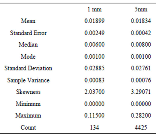
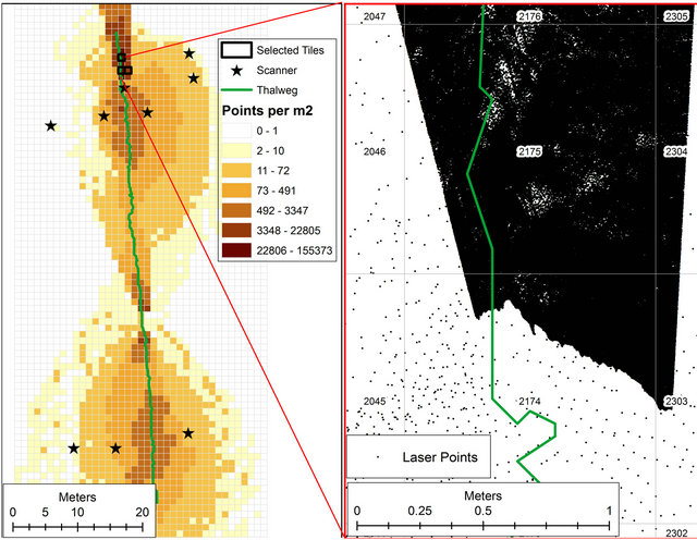
Figure 7. Ground-based LiDAR point density investigation. Left hand-side map shows the spatial variation of the sampling density in square meter cell size grid. The right hand-side map illustrates the differences in point density between tiles. Tile 2174 has 61,912 laser points per square meter while tile 2175 has 155,373 laser points per square meters (both represented by black dots).
with σelev = 0.01). The same variation in elevation represented by standard deviation values can be observed on histograms (Figure 8). Tile 2175 has the largest elevation range (≅ 50 cm) as the gully active headcut is located in this tile. Histogram plots of the distance values to the nearest neighbor depict point density of each plot. The vast majority of the points are within 5 mm of other points.
Experimental semivariograms for each of the three tiles selected were computed using the algorithm gamv available in the Geostatistical Software LIBrary (GSLIB) due to the irregularly spaced nature of the laser points [28]. The lag separation distance (distance between two points used to create the point pair database) and lag tolerance were selected to be 2 cm and 1 cm respectively (2 cm ± 1 cm). The omnidirectional variogram was considered throughout our investigation.
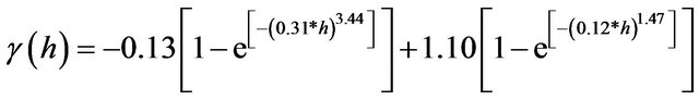
The experimental semivariograms were computed using all the available laser points in each tile with the gamv algorithm (black dots in Figure 9). The theoretical semivariograms were generated using the LevenbergMarquardt optimization algorithm [29] for determining the set of parameters that provides the best fit to the experimental variogram through minimization of the sum of squares of the residuals. Different mathematical models were selected to represent the theoretical semivariogram curves. For tile 2175 a composite Gaussian model was used (Equation (2)).
 (2)
(2)
Variations of the standard Gaussian model were used to generate theoretical semivariogram curves for the remaining two tiles 2304 (Equations (3)) and 2177 (Equation (4)). The three curves of the theoretical semivariograms are plotted in Figure 10. These theoretical semivariograms were considered as reference in the subsequent spatial continuity experiment.
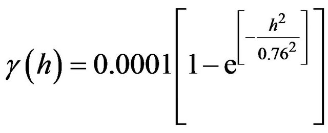 (3)
(3)
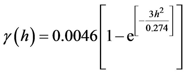 (4)
(4)
Randomly selecting a subset of points for each tile and then evaluating their variogram was utilized to quantify of the influence of the sampling density on the topographic information. Large number of repetitions for the random creation of the subsets was adopted to minimize the odds, and possible influence, of one “bad” selection of points. A Monte Carlo type investigation was performed by creating a series of independent simulations of reduced datasets containing a smaller number of laser points than the original number in each tile. The reduced dataset was generated by randomly selecting laser points based on a pre-defined percentage. A percentage of 100% represents all the laser points available in the tile while a reduced set using a percentage of 50% would yield half of the available points in the tile. For each predefined percentage, a total of 100 independent realize-
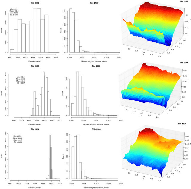
Figure 8. Three tiles selected for the point sampling density investigation. Left hand-side column presents the histograms of elevation values, center column the distance to the nearest neighbor in each of the square meter tile considered, and the right hand-side column three-dimensional grids of each tile.
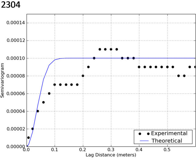
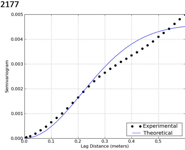
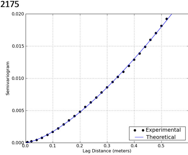
Figure 9. Plots contrasting experimental and theoretical semivariogram for tiles 2175, 2177, and 2304 of irregularly spaced elevation points collected using ground-based laser scanner.
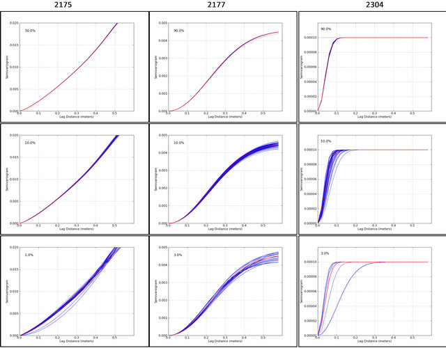
Figure 10. Comparison of theoretical variograms generated using all available data points (red) and reduced dataset (blue). Percentage values indicate the amount of points randomly selected for variance analysis. A total of 100 realizations were performed for each percentage of points considered.
tions were performed (100 independent randomly selected reduced sets). Each reduced set was used in the computation of experimental and theoretical semivariogram curves (Figure 10). Multiple percentage threshold values were used (90%, 80%, 70%, 60%, 50%, 40%, 30%, 20%, 10%, 9%, 8%, 7%, 6%, 5%, 4%, 3%, 2%, and 1% for tile 2177;90%, 80%, 70%, 60%, 50%, 40%, 30%, 20%, 10%, 9%, 8%, and 7% for tile 2304; and 50%, 40%, 30%, 20%, 10%, 9%, 8%, 7%, 6%, 5%, 4%, 3%, 2%, and 1% for tile 2175). Smaller percentage threshold values introduce higher levels of uncertainty represented by the increased variability of the curves.
4. Discussion of Results
The theoretical semivariogram curves generated with reduced data points were quantitatively evaluated by individual comparison to the theoretical semivariogramcurve, obtained using all collected laser points, through the calculation of root mean squared deviation (RMSD) as shown in Equation (5).
 (5)
(5)
In this equation, V100 represents the theoretical semivariogram curve developed using all available laser points, n is the total number of points in the curve (total number of lag interval considered), VP represents theoretical semivariogram curves generated using a reduced dataset with percentage P. A total of 100 RMSD values for each percentage threshold were calculated and averaged. The resulting set of averaged RMSD values are graphically displayed in Figure 11 for each tile.
The three curves display similar shape with the largest discontinuities found in the plot for tile 2304. Points representing the percentage of 10% and 8% yielded higher averaged RMSD values than the point with the lowest number of points (7%). This can be partially explained
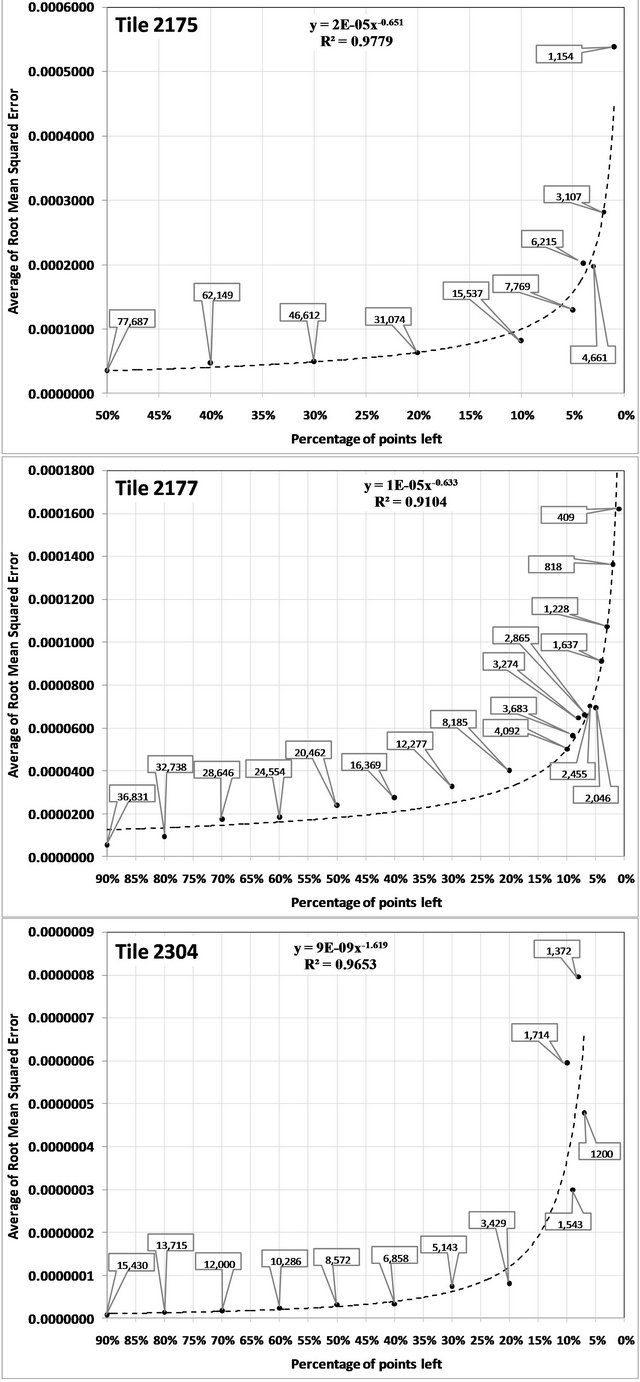
Figure 11. Comparison of the goodness of fit between theoretical variogram using 100% of the available laser points in each tile and 100 realizations of reduced sets of points. Numbers in the callout boxes represent the number of points per square meter left in the tile for each percentage considered.
by the procedure from which a reduced set was created. A standard random sampling technique was used, therefore, it is possible that selected points were not uniformly distributed throughout the tile (forming clusters) and as result, the theoretical variogram curve differs from the reference, yielding large RMSD values. Just a few realizations of clustered points could significantly increase the average value. Nonetheless, despite these two discontinuities it is possible to identify a general trend. The curves start with a gentle slope and as the number of points becomes smaller, curves tend towards to increase rapidly. In other words, results indicate that, in the scale considered, there is an upper threshold of point density where topographic information provided by the LiDAR point cloud does not increase (or increases very little) despite the increased point sampling density. Additionally, it can be observed a positive relationship between this minimum number of points and the tile standard deviation of elevation, as higher sampling densities are needed to topographically describe locations with higher relief, as expected.
To further evaluate the effect of point sampling on topographic information, these curves were used to select three threshold values to reduce the remaining tiles in the survey, 7500, 4000, and 3500 laser points per square meter from tile 2175, 2177, and 2304 respectively. A histogram of the standard deviation of elevation values was used to identify the quartile threshold values. Using these values, the number of laser points in a tile was reduced to the threshold of 7500 laser points per square meter if the standard deviation of elevation was ≥ 0.03617, to 4000 laser points per square meter if the standard deviation of elevation was <0.03617 and ≥ 0.0106, and to 3500 laser points per square meter if the standard deviation of elevation was ≤0.0106. A total of 25 tiles were reduced.
The two point clouds, original and reduced, were converted to Triangular Irregular Network (TIN) format to facilitate volume computations. TIN format was chosen over the conversion of the point cloud into a raster grid to minimize uncertainties caused by interpolation methods. A third TIN, with artificially filled channel, was created by manually digitizing the edges of the gully channel to form a polygon and then subsequent removal of all the laser points within the channel polygon. Through the use of differencing technique, the original and reduced TINs were subtracted from the artificially filled channel TIN yielding volumes estimate of 18.154 m3 and 18.146 m3 respectively. There is a difference of less than 0.04% between the two estimates. Additionally, visual comparison of the thalweg profiles for both datasets confirms the agreement between the original and reduced dataset (Figure 12).In multi-temporal research efforts, it is important to obtain accurate horizontal and vertical characterization of the gully’s thalweg in order to precisely characterize gully changes over time leading to improved understanding of gully evolution.
5. Summary and Concluding Remarks
This study used the concept of semivariogram to quanti-
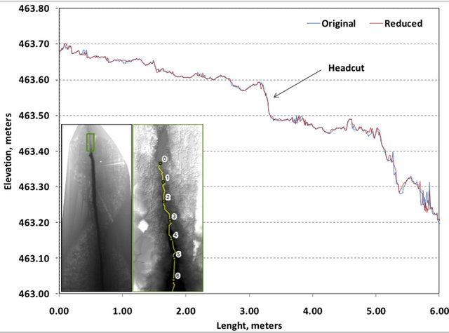
Figure 12. Thalweg topographic profile generated using ground-based LiDAR. Two frofiles are compared: blue profile was generated using all the surveyed points and red profile was generated using a reduced dataset.
tatively investigate the relationship between LiDAR point sampling density and topographic modeling needed to evaluate ephemeral and classic gullies in agricultural fields. The impact of gullies in agricultural fields can be studied at different scales, such as watershed, field, and individual gully scales. In this study, we addressed effects of point sampling density on the topographic information at the individual gully scale.
The gully investigated was partitioned into square meter tiles and the sampling density of each tile was computed by counting the number of laser points in each tile. This experiment revealed a large variation in LiDAR point sampling density throughout the gully. Tiles were ranked by standard deviation of elevation values and partitioned into three groups based on quartile of the histogram elevation values (representing three different topographic characteristics). The tile with the highest number of points in each group was selected for the sensitiveity analysis. Multiple realizations of subsets of randomly selected points at pre-defined percentages were used to identify the minimum point sampling density in which the data set retains the original spatial characteristic. Us- - ing the minimum number of points per square meter thresholds, a reduced point cloud dataset was developed and compared to the original dataset yielding not significant discrepancy. This indicates that data could be collected with smaller sampling density while retaining the original spatial characteristics.
At the fine sampling density required to proper characterize ephemeral gully evolution in agricultural fields, results indicate that well planned surveys could be designed to collect between 3500 to 7500 points per square meter based on the local terrain topographic variability. Such surveys, could significantly expedite data collection without loss of topographic information. It is also important to note that, although results indicated that the reduced dataset did not significantly differ from the originnal dataset in terms of topographic information, and thus these tiles could be considered over-sampled, the reduced tiles represent only a small percentage of the entire dataset. Out of 2085 tiles containing laser points, only 25 were reduced because they had originally more laser points than the defined thresholds. And, out of the 25 reduced tiles only 14 were located in and around the gully channel. Despite the oversampling of 14 tiles in and around the gully channel, still there are 175 tiles (out of 189) located in and around the gully channel that contained fewer points per square meter than the threshold values obtained as result of this study. This is an inherent consequence of the large variation in sampling density.
Although the ideal situation would be to survey gullies with the highest possible sampling density, this is often not practical because sampling density varies with factors such as resolution of the instrument, vertical scan angle, number of overlapping scans, and land coverage. Furthermore, scientific investigation to quantify and to understand the development of ephemeral and classic gullies in agricultural fields over time often requires multitemporal surveys of multiple locations throughout the watershed.
Based on the findings of this study, future field campaigns can be designed to generate consistent datasets with minimum point sampling density considering the different topographic characteristic (3500, 4000, 7500 laser points per square meter). During the field collection the laser scanner is mounted on a tripod that can be elevated allowing the possibility of collecting data far away from the nadir situation (large vertical angles). Collection of data with such large vertical angles leads to lower sampling densities and shadowing when investigating gullies with deep channels. One possible alternative would be to survey the same location using multiple overlapping scans each with lower point density. Although the instrument would be set to collect data at a lower point density, the combined set of scans would yield higher point density. Additionally, the overlapping dataset could be used to evaluate the point cloud by identifying pairs of points with high elevation difference what could be a potential cue to remove anomalies from the data cloud.
The use of ground-based LiDAR for ephemeral and classical gully investigations in agricultural fields is relatively new and research in this field is expected to continue to grow as technology becomes less expensive and new applications are developed. The use of such technology can help in collecting detailed micro-topography information that can be used in many different research areas such as ephemeral and classical gully modeling, soil water depressional storage capacity, terrain roughness measurements, and many others. Continuation of this work will investigate the influence of vegetation canopy and standing crop residue on the laser point sampling density and the derived topographic information.
6. Acknowledgements
The authors would like to acknowledge Don Seale for his indispensible assistance during data collection. Thanks are also due to Howard Miller and Lisa French, at Cheney Lake Watershed, Inc, for contacting and coordinating with local landowners and providing logistic support.
REFERENCES
- W. H. Wischmeier and D. D. Smith, “Predicting Rainfall Erosion Losses,” Agricultural Research Service, Washington DC, 1978, 58 p.
- “CREAMS: A Field-Scale Model for Chemicals, Runoff, and Erosion from Agricultural Management Systems,” In: W. G. Knisel, Ed., USDA Conservation Research Report, No. 26, 1980, p. 640.
- K. G. Renard, G. R. Foster, G. A. Weesies and J. P. Porter, “RUSLE: Revised Universal Soil Loss Equation,” Journal of Soil and Water Conservation, Vol. 46, No. 1, 1991, pp. 30-33.
- R. L. Bingner, R. R. Wells, H. G. Momm, F. D. Theurer and L. D. Frees, “Development and Application of Gully Erosion Components within the USDA AnnAGNPS Watershed Model for Precision Conservation,” Proceedings of the 10th International Conference on Precision Agriculture, Denver, 18-21 July 2010, pp. 18-21.
- Soil Science Society of America, “Glossary of Soil Terms,” Soil Science Society of America, Madison, 2001, p. 134.
- R. M. B. Quadros, C. Wisneiwski and E. Passos, “Modelagem de Canais Incisivos—Revisao,” RA'EGA, Vol. 8, pp. 69-81. (Portuguese)
- J. Casali, J. Lopez and J. Giráldez, “Ephemeral Gully Erosion in Southern Navarra,” CATENA, Vol. 36, No. 1-2, 1999, pp. 65-84.
- D. Woodward, “Method to Predict Cropland Ephemeral Gully Erosion,” CATENA, Vol. 37, No. 3-4, 1999, pp. 393- 399.
- O. Cerdan, V. Souchère, V. Lecomte, A. Couturier and Y. Le Bissonnais, “Incorporating Soil Surface Crusting Processes in an Expert-Based Runoff Model: Sealing and Transfer by Runoff and Erosion Related to Agricultural Management,” CATENA, Vol. 46, No. 2-3, 2002, pp. 189- 205.
- C. Parker, C. Thorne, R. Bingner, R. Wells and D. Wilcox, “Automated Mapping of Potential for Ephemeral Gully Formation in Agricultural Watersheds,” National Sedimentation Laboratory, Oxford, 2007.
- T. Schmid, H. Schack-Kirchner and E. Hildebrand, “A Case Study of Terrestrial Laser-Scanning in Erosion Research: Calculation of Roughness Indices and Volume Balance at a Logged Forest Site,” International Archives of Photogrammetry, Remote Sensing and Spatial Information Sciences, Vol. 36, No. 8, 2004, pp. 114-118.
- R. Perroy, B. Bookhagen, G. Asner and O. Chadwick, “Comparison of Gully Erosion Estimates Using Airborne and Ground-Based LiDAR on Santa Cruz Island, California,” Geomorphology, Vol. 118, No. 3-4, 2010, pp. 288- 300. doi:10.1016/j.geomorph.2010.01.009
- L. A. James, D. G. Watson and W. F. Hansen, “Using LiDAR Data to Map Gullies and Headwater Streams under Forest Canopy: South Carolina,” CATENA, Vol. 71, No. 1, 2007, pp. 132-144. doi:10.1016/j.catena.2006.10.010
- B. D. Collins, K. M. Brown and H. C. Fairley, “Evaluation of Terrestrial LIDAR for Monitoring Geomorphic Change at Archeological Sites in Grand Canyon National Park, Arizona,” U.S. Geological Survey, Open-File Report, 2008, 60 p. http://pubs.usgs.gov/of/2008/1384/
- K. H. Hsiao, J. K. Liu, M. F. Yu and Y. H. Tseng, “Change Detection of Landslide Terrains Using GroundBased LiDAR Data,” 20th ISPRS Congress, Istanbul, 12-23 July 2004.
- J. J. Roering, L. L. Stimely, B. H. Mackey and D. A. Schmidt, “Using DInSAR, Airborne LiDAR, and Archival Air Photos to Quantify Landsliding and Sediment Transport,” Geophysical Research Letters, Vol. 36, No. 19, 2009, Article ID: L19402.
- A. Wehr and U. Lohr, “Airborne Laser Scanning—An Introduction and Overview,” ISPRS Journal of Photogrammetry and Remote Sensing, Vol. 54, No. 2-3, 1999, pp. 68-82. doi:10.1016/S0924-2716(99)00011-8
- R. M. Measures, “Laser Remote Sensing Fundamentals and Applications,” John Wiley & Sons, Inc., Hoboken, 1984.
- S. Wu, J. Li and G. H. Huang, “A Study on DEM-Derived Primary Topography Attributes for Hydrologic Applications: Sensitivity to Elevation Data Resolution,” Applied Geography, Vol. 28, No. 3, 2008, pp. 210-233. doi:10.1016/j.apgeog.2008.02.006
- Q. Guo, W. Li, H. Yu and O. Alvarez, “Effects of Topographic Variability and Lidar Sampling Density on Several DEM Interpolation Methods,” Photogrammetric Engineering and Remote Sensing, Vol. 76, No. 6, 2010, pp. 701-712.
- P. I. Curran and P. M. Atkinson, “Geostatistis and Remote Sensing,” Progress in Physical Geography, Vol. 22, No. 1, 1998, pp. 61-78.
- P. K. Kitanidis, “Introduction to Geostatistics: Application in Hydrogeology,” Cambridge University Press, Cambridge, 1997.
- I. Clark, “Practical Geostatistics,” Applied Science, New York, 1979.
- C. E. Woodcock, A. H. Strahler and D. L. B. Jupp, “The Use of Variograms in Remote Sensing: II. Real Digital Images,” Remote Sensing of Environment, Vol. 25, No. 3, 1988, pp. 349-379. doi:10.1016/0034-4257(88)90109-5
- J. C. Davis, “Statistics and Data Analysis in Geology,” John Wiley and Sons, New York, 2002.
- E. H. Isaaks and R. M. Srivastava, “Applied Geostatistics,” Oxford University Press, New York, 1989.
- S. Soudarissanane, R. Lindenbergh, M. Menenti, P. Teunissen and T. Delft, “Incidence Angle Influence on the Quality of Terrestrial Laser Scanning Points,” Proceedings ISPRS Workshop Laser Scanning, 1-2 September 2009, Paris, pp. 183-188.
- C. V. Deutsch and A. G. Journel, “GSLIB: Geostatistical Software Library and User’s Guide,” Oxford University Press, New York, 1998, 369 p.
- K. Levenberg, “A Method for the Solution of Certain NonLinear Problems in Least Squares,” The Quarterly of Applied Mathematics, Vol. 2, No. 2, 1944, pp. 164-168.
NOTES
*Corresponding author.