Theoretical Economics Letters
Vol.3 No.2(2013), Article ID:30812,11 pages DOI:10.4236/tel.2013.32018
The Impact of Bank Health on Coordination among Creditors
College of Economics, Nihon University, Tokyo, Japan
Email: toyofuku.kenta@nihon-u.ac.jp
Copyright © 2013 Kenta Toyofuku. This is an open access article distributed under the Creative Commons Attribution License, which permits unrestricted use, distribution, and reproduction in any medium, provided the original work is properly cited.
Received January 23, 2013; revised February 20, 2013; accepted March 18, 2013
Keywords: Coordination Failure; Heterogeneous Bank Financing; Global Game
ABSTRACT
We investigate how the health of a relationship bank impacts upon coordination among creditors and how it affects the firm’s behavior. We show that if the relationship bank is healthy, creditors coordinate each other and the firm takes an efficient action but if it becomes financially distressed, a coordination problem arises ex post and the inefficient liquidation of the firm’s projects may occur. This coordination failure, in turn, increases the interest payments ex ante so that the firm is more likely to choose an inefficient action.
1. Introduction
This paper investigates how the health of a firm’s relationship bank affects the actions of firms and the coordination of creditors. In line with Modigliani and Miller’s [1] seminal contribution, not only the financial structure of the firm but also the firm’s sources of capital are irrelevant in terms of firm valuation. However, in practice, because of asymmetric information between agents, transaction costs, and the presence of social or traditional institutions, it is costly for the firm to switch creditors, especially away from its existing relationship bank.
The pros and cons of relationship banking have been discussed in many studies (Petersen and Rajan [2], Boot [3], Boot and Thakor [4], and Berger and Udell [5])1. Within these studies, it is argued that the close ties between the relationship bank and the firm potentially provide improvements in information production and monitoring, assist in the renegotiation of contracts, and thus increase the availability of loans to the firm. However, this also grants monopoly power to the relationship bank, and thus the firm may face an ex post hold-up problem.
Moreover, these relations can be adversely affected when the relationship bank becomes financially distressed. For example, Gibson [6,7] concluded that publicly listed Japanese firms with ties to lower-rated relationship banks typically spent less on investment in the early 1990s than firms associated with higher-rated banks2. Similarly, Bae et al. [8] found that when relationship banks failed during the 1997-1998 Korean banking crisis, the stock returns of the borrowing firms generally fell3.
However, in practice, many firms, particularly in Europe and Asia, borrow from several banks. For instance, Ongena and Smith [9] showed that large European firms usually borrow from eight or more banks, while Miyakawa [10] found that the typical Japanese firm obtained funds from 9.8 banks in 1999. Detragiache et al. [11] showed that the benefit of establishing multiple banking relationships is to mitigate the liquidity risk in spite of higher transaction costs4.
In the multiple banking relationships, one bank acts as a relationship bank and other banks act as “arm’s length” lenders (Bannier [12]). Unfortunately, the overriding prevalence of heterogeneous multiple bank financing has received scant attention in the theoretical literature. This is partly because of a technical difficulty faced in this sort of analysis. That is, when incorporating the coordination problem between a relationship bank and other arm’s-length banks, we face the problem of multiple equilibria. With multiple equilibria, because it is impossible to determine which equilibrium is achieved, we cannot generally determine how the coordination problem affects the firm manager’s incentives and the nature of the ex ante financial contract. However, recent progress in the literature on equilibrium selection, especially the notion of the global game, enables us to better analyze these issues. This is because when we introduce incomplete information and strategic complementarities among players into the model, we can obtain a unique equilibrium solution.
There has been much recent research on how coordination failure among creditors affects the financial contract based on the concept of the global game (Morris and Shin [20], Hubert and Schafer [21]). Recently, the coordination problem arising from heterogeneous multiple bank financing has also been the subject of some attention by Bannier [12]. Bannier [12] extended the model in Corsetti et al. [22] using the asymmetric global game and derived a unique equilibrium, showing that in some circumstances because of the information advantages of the relationship bank, heterogeneous multiple bank financing urges the coordination between the relationship bank and the other arm’s-length creditors and thereby leads to fewer inefficient credit decisions than either monopoly relationship lending or homogeneous multiple bank financing.
This paper, by incorporating the health of the relationship bank into the model, investigates how the relationship bank’s health affects the coordination between itself and the firm’s other creditors and how this expost coordination problem affects the ex ante efficiency of the firm’s actions. Our main findings are as follows. First, as the relationship bank becomes financially distressed interest payments by the firm to both the relationship bank and its other creditors increase because of coordination failure. This is because as the relationship bank becomes distressed, it desires the firm to undertake riskier actions whereas the other creditors want the firm to undertake safer actions. Thus, a coordination problem arises in the interim period and the other creditors are then more likely to withdraw their loans from the firm. Therefore, the poor health of the relationship bank induces the inefficient liquidation of the firm’s projects and this reduces the economy’s ex post efficiency. Second, this increased ex post inefficiency also reduces the ex ante efficiency of the firm’s actions. This is because the higher interest payments made to the relationship bank and other creditors encourage the firm to select inefficient and riskier projects. Overall, as the financial health of the relationship bank deteriorates, the efficiency of the economy also declines from both an ex ante and expost point of view through the increased coordination failure found among creditors.
The remainder of the paper is structured as follows. Section 2 describes the model to be used. In Section 3, we consider project choice by the firm. In Section 4, we derive the creditor’s decision and derive the equilibrium strategies of the relationship bank and the firm’s other creditors. In Section 5, we determine the interest payments by the firm to both the relationship bank and its other creditors. In Section 6, we investigate the comparative statics and derive how the health of the relationship bank affects the coordination among creditors and the firm’s choice of project. Section 7 concludes the paper.
2. The Model
We assume there are three periods,  and three types of agents, a firm, a relationship bank, and a continuum of other creditors. The firm has a fixed scale technology that requires one unit of capital at
 . The firm also has no wealth and borrows
  units from the relationship bank and
  units from its other creditors. For the relationship bank, there is an outstanding debt,
  at
at .
.
At , project quality
  is realized and the relationship bank and the other creditors receive a signal of the prospects of a project as
  and
and , respectivelywhere
  with
with  and
and
 with
with
 .
.
We assume  is i.i.d. across the other creditors and
  and
and  are independent of each other and
 . We also assume that
  such that the relationship bank has the ability to acquire relatively more precise information about the firm.
Given the signals concerning the firm’s project, the creditors decide whether to continue or withdraw their loans from the firm. If the relationship bank withdraws its loans, it receive a liquidation value  and the other creditors’ liquidation value is
 . Let
. Let  be the amount of loans that are continued at
  and
and  be the proportion of creditors that continue their loans. At
 , knowing
 , the firm’s manager decides whether to implement the safe project or the risky project. At
 , the firm’s final output is realized. Then the relationship bank demands repayment of
  and each other creditor demands a repayment of
 , both of which are determined at
 . If the project generates sufficient cash to meet the repayment demands of the firm’s creditors, the firm then receives the residual output.
The payoff of the project thus depends on the decisions of both the manager and the creditors; that is, whether the manager chooses the safe project or the risky project and how many creditors continue their loans. Consider if project quality  is realized at
  and the amount
  of loans are continued at
 . When the firm chooses the safe project, the firm’s output at
  is
is  with a probability of one (certainty) where
  and
and . That is, the firm’s output increases when more creditors continue at
  (strategic complementarity). Alternatively, when the firm chooses the risky project, the firm’s output is
  with a probability of
  and 0 with a probability of
  where
where . That is, it is assumed that choosing the safe project is always efficient for every value of
 . If the final output does not meet the total repayments of creditors, the firm goes bankrupt at
  and the creditors divide the output in proportion to the size of their loans to the firm. We assume that the liquidation value of the asset is 0 at
 .
.
3. Project Choice by the Firm
In this section, we consider the firm’s incentives. The condition for the safe project to be chosen depends on the number of creditors willing to continue their loans until . Let
. Let  and
and  be the amount of creditors and the total amount of repayment when the relationship bank continues (withdraws) at
 . Then,
When the firm chooses the safe project, the final output at  is
is  with probability one if the project quality
  is realized at
 . Let
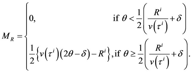
. Let  be the firm’s payoff at
  when it chooses the safe project and the relationship bank rolls the loan over. Then,
  can be written as:
Next, consider the case in which the firm chooses the risky project. In this case, given the project quality  is realized with probability
  and 0 with probability
 . Then, as in the previous case, let
  be the firm’s expected payoff at
  when the firm chooses the risky project. Then,
  can be written as follows:
The firm chooses the safe project if . That is, the firm chooses the safe project at
  when the following inequality is satisfied.
 (1)
(1)
Obviously, this condition is affected by whether the relationship bank continues its loan. We further investigate this condition in the next section.
4. The Creditors’ Decision
In this section, we investigate the choice of the creditors in whether to continue or withdraw their loans at . Under the settings of this model, we can characterize this as a switching strategy whereby the relationship bank withdraws (continues) the loan if it observes the signals below (above)
  and the other creditors withdraw (continue) their loans if they observe the signals below (above)
  5. In this section, we first derive the equilibrium switching strategies for both types of creditors. We then consider how the health of the relationship bank affects the coordination of creditors and the risk-taking of the firm.
4.1. The Other Creditors’ Choice
In this subsection, we derive the equilibrium switching strategies of the other creditors (not the relationship bank). The payoffs for the other creditors depend on three factors: that is, how many creditors continue their loans at , whether the relationship bank continues its loan, and the project the firm chooses. First, the proportion of other creditors continuing their loans at
 , is given by those that receive private information higher than
 . Note that
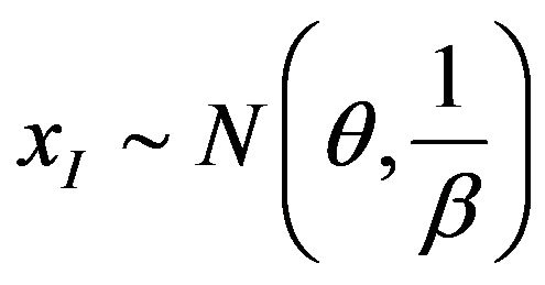 ,
,
where  denotes the cumulative normal distribution.
Given that  increases as
  increases, by definition,
  is also increasing in
 . Let
. Let  denote the threshold above which the firm chooses the safe project when the relationship bank continues (withdraws) its loan. Then, we can derive the following lemma.
Lemma 1. When  and
and  are small and the degree of strategic complementarity is small, the firm is more likely to choose the safe project.
(Proof) See Appendix 1.
Lemma 1 indicates that when  is large, or
  is small, the firm is more likely to choose the risky project. Moreover, given the same number of creditors who continue their loan, the payoff of the firm becomes smaller as the degree of the strategic complementarity becomes larger. Thus, the firm can obtain more when it chooses the risky project than when it chooses the safe project.
Next, we calculate the expected payoff for the other creditors at . As their payoffs are affected by whether the relationship bank continues its loan and which project the firm chooses, we can categorize their payoffs into four cases.
1) The case when the relationship bank continues and the firm chooses the safe project
In this case, when the creditors receive a signal , they consider that
  is distributed according to
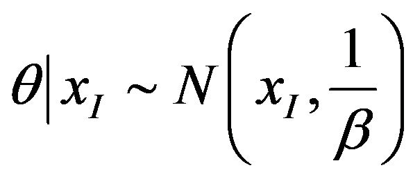 . As
. As  and
and the creditors consider that
  is distributed according to
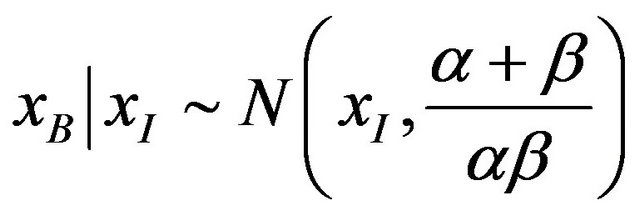 .
.
Thus, creditors receiving the signal  believe that the relationship bank will continue with probability
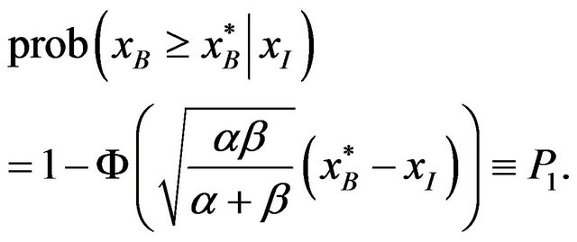
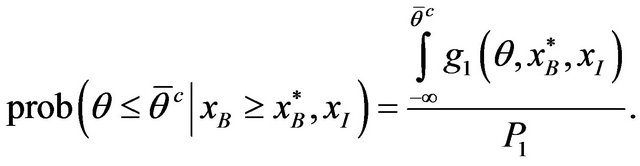
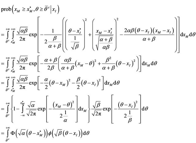
In addition, the probability they assign to the firm choosing the safe project given that the relationship bank continues is6
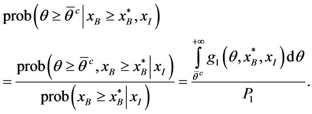
where
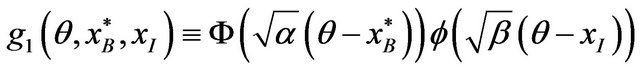 .
.
In this case, the proportion of loans that are continued becomes . Let
. Let  be the expected payoff of each other creditor. Then,
Note that when , the firm goes bankrupt and creditors receive the output in proportion to their stake in the firm.
2) The case when the relationship bank continues and the firm chooses the risky project
In this case, the probability that other creditors assign to the firm choosing the risky project given that the relationship bank continues is
In this case, . Let
. Let  be the expected payoff of each other creditor. Then,

3) The case when the relationship bank withdraws and the firm chooses the safe project
In this case, when creditors receive a signal , they consider that the relationship bank withdraws with probability
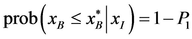 .
.
In addition, the probability that they assign to the firm choosing the safe project given that the relationship bank withdraws is
where . In this case,
 . Let
. Let  be the expected payoff of each other creditor. Then,
4) The case when the relationship bank withdraws and the firm chooses the risky project
In this case, the probability that creditors assign to the firm choosing the risky project given that the relationship bank withdraws is
In this case, as in the previous case, . Let
. Let  be the expected payoff of each other creditor. Then,
Denoting by  the expected payoff of creditors when they receive a signal
 , then,
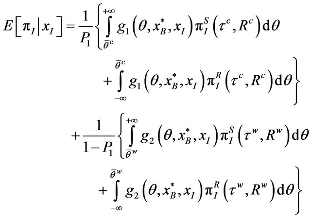 (2)
(2)
Then, the trigger value  is determined so that creditors are indifferent between withdrawing and continuing their loans:
Then, we can derive the following proposition.
Proposition 1.  is strictly increasing in
  and thus
  is uniquely determined.
(Proof) See Appendix 3.
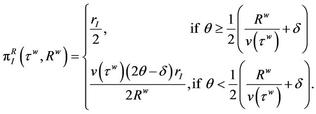
4.2. The Relationship Bank’s Choice
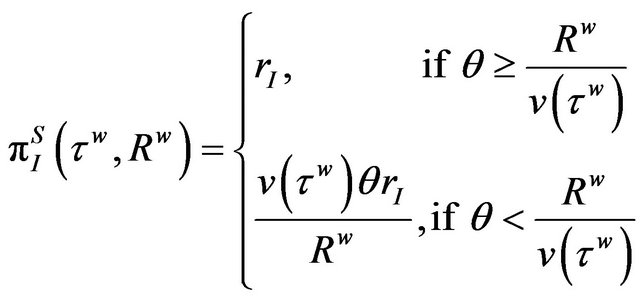
Next, consider the relationship bank’s switching strategy. The payoff for the relationship bank when it continues its loan depends on how many of the other creditors continue their loans, the project the firm chooses, and the amount of outstanding debt, . First, when the firm chooses the safe project, the expected payoff for the relationship bank,
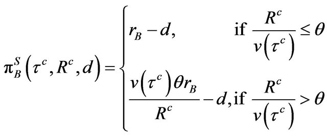
  , can be described as follows:
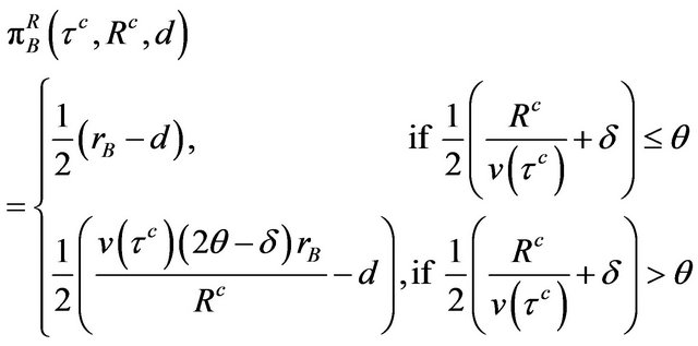
Next, consider the case when the firm chooses the risky project. Let  be the expected payoff for the relationship bank. Then,
Comparing  with
with , we derive the following lemma.
Lemma 2. When 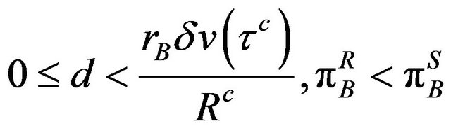 holds for all
 . When
  holds when
  and
and  holds when
  where
where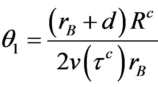 .
.
Lemma 2 indicates firstly that the relationship bank wants the firm to undertake the safe project when the bank is prudent (i.e.,  is small), and secondly that when
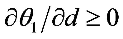 , as the relationship bank becomes less prudent and
  is small, it becomes better off if the firm undertakes the risky project. Therefore, from Lemma 2, when the relationship bank is less prudent, the relationship bank wants the firm to select the risky project, and this incentive lies contrary to that of the other creditors.
Next, consider the optimal switching strategy of the relationship bank. When the relationship bank receives a signal , it considers
  to be distributed as
 . Then, if the relationship bank continues its loan, it considers that the firm will choose the safe project with
 .
.
Given that under the optimal switching strategy the relationship bank receives the same expected payoff for continuing and withdrawing,  is determined to satisfy the following equation.
 (3)
(3)
Then, we can derive the following proposition.
Proposition 2. As the LHS of (3) is strictly increasing,  is uniquely determined.
(Proof) See Appendix 4.
From Propositions 1 and 2, we derive the equilibrium switching strategies of the relationship bank and the other creditors at .
.
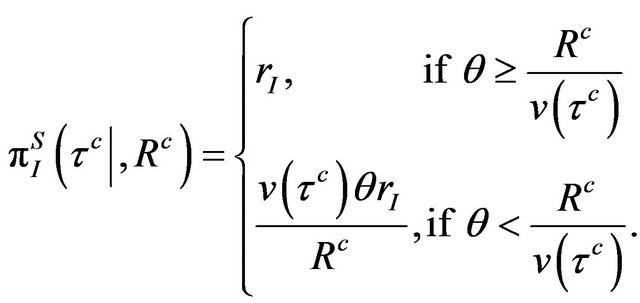
5. The Determination of rI and rB
In this section, given the equilibrium strategies of creditors at , we discuss how
  and
and  are determined at
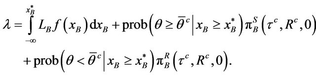
 . First, consider the case of
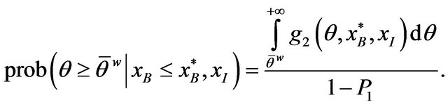
 . As creditors obtain the liquidation value if they receive a signal below
  is determined to satisfy the following equation:
 (4)
(4)
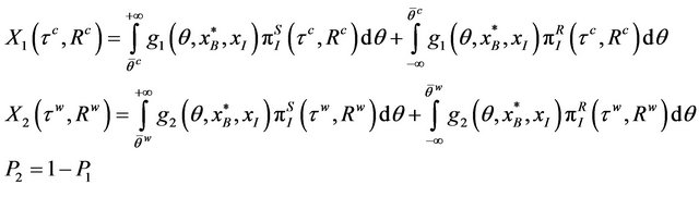
The first term on the RHS in (4) denotes the expected liquidation value at , while the second term is the expected payoff when both the relationship bank and the other creditors continue their loans and the firm chooses the safe project.
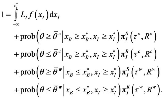
Next, consider the case of .
.  is determined so as to satisfy
(5)
Note that, in determining the level of , the firm is unconcerned about the amount of outstanding debt held by the relationship bank. In other words, the level of
  is determined regardless of the level of
 . Therefore, the second and third terms in (5) are included
 and
and , not
, not 
and . In sum, the equilibrium of this model
 is solved by (1), (2), (3), (4), (5).
6. Comparative Statics
In this section, we investigate how the prudence of the relationship bank affects the ex ante and ex post efficiency of the model economy. To prove this problem, we analyze the comparative statics of the model, especially by changing the size of . To derive this, we firstly consider the relation between
  and
and . Then, we can derive the following proposition7.
Proposition 3.  if
if  and
and  if
if .
.
(Proof) See Appendix 5.
This proposition indicates that when  is small, such that
  holds, the increase in
  increases the level of
 . That is, when the relationship bank is prudent, but its financial condition worsens, it is more likely to withdraw its funds from the firm. Conversely, when
  is large, the relationship bank cannot gain a positive expected payoff if the firm chooses the safe project, such that
  holds. Consequently, when
  becomes larger, the relationship bank sets
  lower.
Next, consider the relation between  and
and . In terms of this, we can derive the following proposition.
Proposition 4. When  is small or
  is small,
 . Otherwise,
 .
.
(Proof) See Appendix 6.
Concerning the relation between  and
and , the other creditors are affected by the relationship bank’s decision in two ways. Suppose the relationship bank decreases
 . First, because the relationship bank assigns a greater probability to continuing its loan, the decision informs the good state of the firm to the other creditors. This is because the relationship bank has an information advantage over the other creditors8. Given that there exists a strategic complementarity between the other creditors and the relationship bank about the return from the project (i.e.,
 ), this effect brings about a greater payoff for each of the creditors. Second, the decrease in
  increases the probability of the firm choosing the risky project. In this case, creditors receive the payoff
  which is less than
 . Thus, if the first positive effect outweighs the second negative effect,
  also decreases (i.e.,
 ). On the other hand, if the second effect outweighs the first effect,
  increases (i.e.,
 ). Then, as Proposition 3 suggests, if the relationship bank is in the region where it wants the firm to undertake the risky project, the other creditors should set
  in the opposite direction to
 .
.
Then, from Propositions 3 and 4, we can immediately derive the following proposition.
Proposition 5. When . Otherwise,
 .
.
This proposition indicates that when the relationship bank becomes less prudent, creditors are more likely to withdraw their loans. This is because, as the previous arguments suggest, when  becomes larger, the relationship bank wants the firm to choose the risky project, unlike the other creditors. In sum, if the relationship bank has outstanding debt at the starting period, it breaks the coordination between the relationship bank and the other creditors, and thus early liquidation of the project may take place. In Corsetti et al. [22] and Bannier [12], the existence of a single large stakeholder motivates the numerous other small creditors to coordinate their choices, as derived from the ability of a large stakeholder to acquire information about the firm more precisely. However, in this model, the existence of the relationship bank brings about both a positive and negative effect on the firm’s other stakeholders (here, other creditors). This difference arises because in this analysis, the firm can choose a safe or a risky project, and, due to the existence of the outstanding debt of the relationship bank, the criteria on which the project choice is based differ between the relationship bank and other creditors.
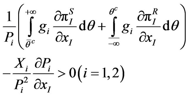
Finally, we derive the following proposition.
Proposition 6. Suppose  is large. When
  is large,
 . When d is small,
  .
.
(Proof) See Appendix 6.
This proposition indicates that when the relationship bank is not prudent, the firm is more likely to select a risky project. The intuition behind this is as follows. Suppose  is small so that the other creditors have the large stakes of the firm. Then, as
  becomes larger, the coordination problem among creditors arises at
  and thus more other creditors withdraw at
 . This, in turn, affects the determination of
  and
and . That is, since
 ,
,  should be increased. As Lemma 1 denotes, the firm is more likely to choose the risky project as
  increases. Therefore, the increase in
  shifts
  and
and  higher. On the other hand, when
  is large so that the relationship bank holds the large stakes of the firm, then as Proposition 3 denotes, it sets
  lower when
  is large. This, in turn, urges the firm to undertake an inefficient risky project. Therefore, regardless the size of
 , the ex ante efficiency of this economy is deteriorated as the relationship bank becomes less prudent.
This proposition therefore sheds light on the dark side of relationship banking. Proposition 5 shows, when it is difficult for borrowers to switch their relationship bank, the availability of loans decreases because of the coordination failure between the relationship bank and the continuum of smaller creditors. In other words, the health of the relationship bank can affect the ex post coordination between the relationship bank and smaller creditors, which in turn affects the ex ante financial condition of borrowers. Therefore, even if two firms have similar technology available to produce the same output and identical financial positions, one firm will be able to borrow more easily because its relationship bank is financially healthier than that of the other firm.
7. Conclusions
This paper investigated how the health of a relationship bank affects the coordination between the relationship bank and other creditors and how the ex post coordination problem affects the ex ante efficiency of the firm’s actions. Our main findings are as follows. First, as the relationship bank becomes more financially distressed, it desires the firm to take risky actions while other creditors require the firm to take safe actions, and thus a coordination problem arises in the interim period. Therefore, the poor health of the relationship bank induces the inefficient liquidation of the firm’s project and thereby reduces the expost economic efficiency. Second, the presence of expost inefficiency also reduces the ex ante efficiency of the firm’s actions because the higher interest payments to the relationship bank and other creditors encourage the firm to choose the inefficient and risky project. These conclusions shed light on the dark side of relationship banking and provide important implications about the efficiency of multiple yet asymmetric bank financing arrangements.
To simplify our arguments, we assumed the liquidation values for both types of creditors are given. However, it would be interesting to construct a framework in which the liquidation value is determined endogenously and is affected by the coordination of creditors. This is left for future research.
REFERENCES
- F. Modigliani and M. Miller, “The Cost of Capital, Corporation Finance and the Theory of Investment,” American Economic Review, Vol. 48, No. 3, 1958, pp. 261-297.
- M. A. Petersen and R. G. Rajan, “The Benefits of Lending Relationships: Evidence from Small Business Data,” Journal of Finance, Vol. 49, No. 1, 1994, pp. 3-37. doi:10.1111/j.1540-6261.1994.tb04418.x
- A. Boot, “Relationship Banking: What Do We Know,” Journal of Financial Intermediation, Vol. 9, No. 1, 2000, pp. 7-25. doi:10.1006/jfin.2000.0282
- A. Boot and A. Thakor, “Can Relationship Banking Survive Competition,” Journal of Finance, Vol. LV, No. 2, 2000, pp. 679-713. doi:10.1111/0022-1082.00223
- A. Berger and G. Udell, “Relationship Lending and Lines of Credit in Small Firms Finance,” Journal of Business, Vol. 68, No. 3, 1995, pp. 351-382. doi:10.1086/296668
- M. S. Gibson, “Can Bank Health Affect Investment? Evidence from Japan,” Journal of Business, Vol. 68, No. 3, 1995, pp. 281-308. doi:10.1086/296666
- M. S. Gibson, “More Evidence on the Link between Bank Health and Investment in Japan,” Journal of the Japanese and International Economies, Vol. 11, No. 3, 1997, pp. 296-310. doi:10.1006/jjie.1997.0379
- K. H. Bae, J. K. Kang and C. W. Lim, “The Value of Durable Bank Relationships: Evidence from Korean Banking Shocks,” Journal of Financial Economics, Vol. 64, No. 2, 2002, pp. 181-214. doi:10.1016/S0304-405X(02)00075-2
- S. Ongena and D. Smith, “What Determines the Number of Bank Relation-ships? Cross-Country Evidence,” Journal of Financial Intermediation, Vol. 9, No. 1, 2000, pp. 26-56. doi:10.1006/jfin.1999.0273
- D. Miyakawa, “How Does the Stability of Loan Relation Depend on Its Duration? Evidence from Firmand BankLevel Data,” DBJ Discussion Paper Series No. 0903, 2009.
- E. Detragiache, P. Garella and L. Guiso, “Multiple versus Single Banking Relationships: Theory and Evidence,” Journal of Finance, Vol. 55, No. 3, 2000, pp. 1133-1161. doi:10.1111/0022-1082.00243
- C. Bannier, “Heterogeneous Multiple Bank Financing: Does It Reduce Inefficient Credit-Renegotiation Incidence,” Financial Markets and Portfolio Management, Vol. 21, No. 4, 2007, pp. 445-470. doi:10.1007/s11408-007-0062-6
- N. Yamori and A. Murakami, “Does Bank Relationship Have an Economic Value? The Effect of Main Bank Failure on Client Firms,” Economics Letters, Vol. 65, No. 1, 1999, pp. 115-120. doi:10.1016/S0165-1765(99)00133-0
- M. Hori, “Does Bank Liquidation Affect Client Firm Performance? Evidence from a Bank Failure in Japan,” Economics Letters, Vol. 88, No. 3, 2005, pp. 415-420. doi:10.1016/j.econlet.2005.05.007
- S. Ongena, C. S. David and D. Michalsen, “Firms and Their Distressed Banks: Lessens from the Norwegian Banking Crisis,” Journal of Financial Economics, Vol. 67, No. 1, 2003, pp. 81-112. doi:10.1016/S0304-405X(02)00232-5
- R. Elsas, “Empirical Determinants of Relationship Lending,” Journal of Financial Intermediation, Vol. 14, No. 1, 2005, pp. 32-57. doi:10.1016/j.jfi.2003.11.004
- L. A. Farinha and J. A. C. Santos, “Switching from Single to Multiple Bank Lending Relationships: Determinants and Implications,” Journal of Financial Intermediation, Vol. 11, No. 2, 2002, pp. 124-151. doi:10.1006/jfin.2001.0328
- K. Ogawa, E. Sterken and I. Tokutsu, “Why Do Japanese Firms Prefer Multiple Bank Relationship? Some Evidence from Firm-Level Data,” Economic Systems, Vol. 31, No. 1, 2007, pp. 49-70. doi:10.1016/j.ecosys.2006.08.002
- K. Ogawa, E. Sterken and I. Tokutsu, “Multiple Bank Relationships and the Main Bank System: Evidence from a Matched Sample of Japanese Small Firms and Main Banks,” The Economics of Imperfect Markets: The Effects of Market Imperfections on Economic Decision-Making, 2009, pp. 73-90.
- S. Morris and H. Shin, “Coordination Risk and the Price of Debt,” European Economic Review, Vol. 48, No. 1, 2004, pp. 133-153. doi:10.1016/S0014-2921(02)00239-8
- F. Hubert and D. Schafer, “Coordination Failure with Multiple-Source Lending, the Cost of Protection against a Powerful Lender,” Journal of Institutional and Theoretical Economics, Vol. 158, No. 2, 2002, pp. 256-275. doi:10.1628/0932456022975394
- G. Corsetti, A. Dasgupta, S. Morris and H. S. Shin, “Does One Soros Make a Difference? A Theory of Currency Crises with Large and Small Traders,” Review of Economic Studies, Vol. 71, No. 1, 2004, pp. 87-114. doi:10.1111/0034-6527.00277
Appendix 1: Proof of Lemma 1
From (1),  is determined so as to satisfy
 (6)
(6)
Given . In addition,
 holds. When the degree of strategic complementarity is large (i.e.,
  and
and ),
),
becomes small. Then,  holds. On the other hand, when
  is large so that
  is large, from (5),
  holds. (q.e.d.)
Appendix 2: The Derivation of 
(q.e.d.)
Appendix 3: Proof of Proposition 1
First, we define the three parameters.
Then, we can derive the following equation.
 (7)
(7)
From the definition of  and
and ,
,  and
and . In addition, as
 .
.
Next, as
 when
when  but
but  may be negative when
 . Then, note that
  is increasing in
  so that
  is larger when
  than when
 ,
,
holds.
Additionally, as
 when
when  but
but  may be negative when
 . However, when
  is large,
holds such that
Finally, although , by assuming strategic complementarity
 ,
,
holds. Therefore  and, by Corsetti et al.
(2004),  is uniquely determined. (q.e.d.)
Appendix 4: Proof of Proposition 2
When  increases,
  decreases. In addition, the increase in
  increases
 , which rises
  and
and . Thus, the RHS of (3) is strictly increased in
 . (q.e.d.)
Appendix 5: Proof of Proposition 3
By totally differentiating (3) with respect to , we can derive
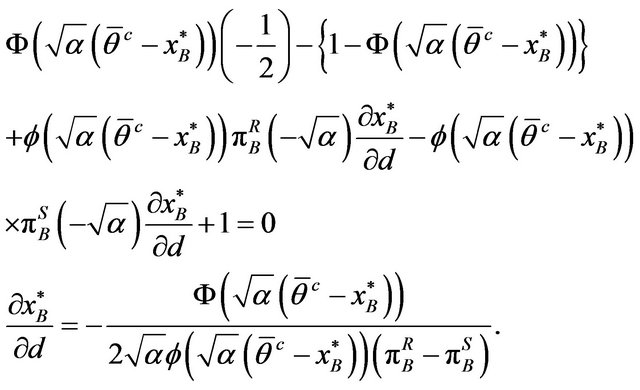
Thus,  if
if  and
and  if
if . (q.e.d.)
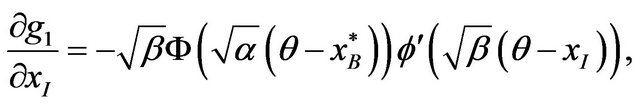
Appendix 6: Proof of Proposition 4
For the proof, we consider how  affects
  because
 is determined by the level of
 .
.
First, we differentiate  and
and  with
with .
.
Next, obviously,
This inequality denotes that, when  becomes higher, the probability that the relationship bank continues its loan becomes lower and thus the payoff
  is less likely to be realized. Further,
That is, as the higher  decreases the range of
  over which the firm chooses the risky project, the second term in the first bracket on the RHS of (2) becomes much smaller than the first term. Conversely, given
 , the second term on the RHS becomes higher. However, as

when  is small such that
  is satisfied. In this case, as
 . On the other hand, when
  is large so that
  is satisfied,
  and thus
  holds. (q.e.d.)
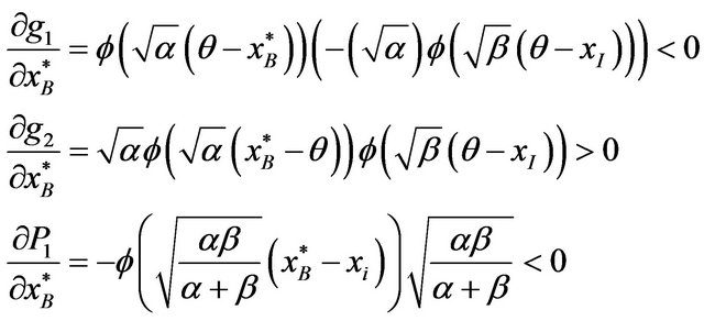
Appendix 7: Proof of Proposition 6
Suppose  is large. From (5),
  increases as
  increases. Thus, when
 . Next consider
 . Given
  when
when  is large, the
NOTES
*I thank Sumio Hirose, Mami Kobayashi and the seminar participants at Nihon University for their helpful comments. This research is supported by a grant-in-aid from Zengin Foundation for Studies on Economics and Finance. Any remaining errors are our responsibility.
1For a discussion on this issue, see Boot [3].
2Yamori and Murakami [13] and Hori [14] also consider how a bank failure affects the performance of client firms.
3In contrast, Ongena et al. [15] argued that there were no significant effects of bank failures on the borrowing firm’s stock returns.
4Ongena and Smith [9], Elsas [16] and Miyakawa [10] consider the stability of loan relations between firms and banks. Farinha and Santos [17] and Ogawa et al. [18] consider the determinants of the multiple banking relationships. In addition, Ogawa et al. [19] show that Japanese firms in the early 2000s increase their number of bank relations to diversify the liquidity risk.
5Corsetti et al. [22] have shown that these switching strategies are unique equilibrium strategies in asymmetric global games. Therefore, we focus on the derivation of the equilibrium switching strategies.
6For the derivation of the numerator on the RHS, see Appendix 2.
7It is assumed that  holds.
8Of course, this effect is strengthened if  increases.